analyzing the coffee addiction habit of the author is an opportunity to reflect on probabilistic thinking and Bayesian decision analysis.
coffee drinking habit
Coffee is the most popular drink in the world and in the right dose it gives our body various benefits. But coffee, as we all know, contains caffeine, a substance which must not be abused in order not to incur a series of side effects which in most cases are minor but in others may involve health risks (nervousness, insomnia , loss of appetite, damage to the cardiovascular system).
Some studies define that the ideal amount of coffee should not exceed 400 milligrams per day, the equivalent of four cups, for an adult man without any particular health problems.
The author is a coffee lover, maybe a coffee addicted. He has an heavy coffee drinking habit that in some case go beyond the daily ideal number of cups.
This post studies the problem of coffee consumption, taken from the author’s daily life, using probabilistic analysis tools. The goal is to outline a problem analysis methodology rooted in probabilistic thinking.
one informal point of view …
Suppose an informed person gives a description of the habit of drinking coffee.
The provided statement is: the author drinks between 1 and 7 cups of coffee a day .
This description may be valid in an informal conversation, but it is not if we want to study the phenomenon of the author’s coffee consumption.
A probabilistic formulation of the informal sentence above shall define:
the possible values that the consumption phenomenon can take in terms of cups of coffee;
the probability of each of these values;
assumptions about the coffee consumption phenomenon along the day sequence.
According to this schema, the probabilistic translation of the sentence could be: the author can drink from 1 to 7 coffees every day, the number of cups per day is equally likely and it is independent of the cups taken the day before.
… formalized in a uniform distribution
In probability theory and statistics, the discrete uniform distribution is a probability distribution wherein a finite number of values are equally likely to be observed; every one of n values has equal probability 1/n.
Another way of saying “discrete uniform distribution” would be “a known, finite number of outcomes equally likely to happen”. \[cups \sim Unif(1,7)\]
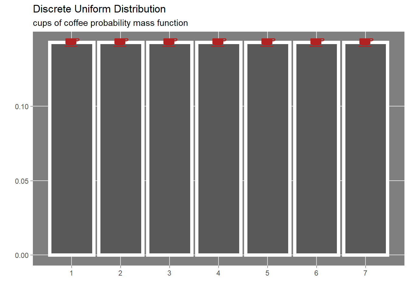
In order to understand what is the meaning of the probabilistic definition, a random draw from the uniform distribution is displayed in the following graph covering last 3 months.
The above visualization of the uniform description of the coffee drinking habit shows how data points (cups) are distributed evenly from 1 to 7 cups a day and no data point is allowed outside this boundary.
but this is what the person questioned meant? or the natural and informal language used has been misleading?
another simple point of view …
Suppose another informed person gives a different description of the habit of drinking coffee.
The provided statement is: the author drinks 4 coffees a day on average.
As before the informal description has to be translated in probabilistic terms which precisely define the uncertainty. the count of coffee cups drunk by the author in a day has a constant average rate of 4 cups a day, the number of cups each day is equally likely and it is independent of the cups taken the day before.
… formalized in a poisson distribution
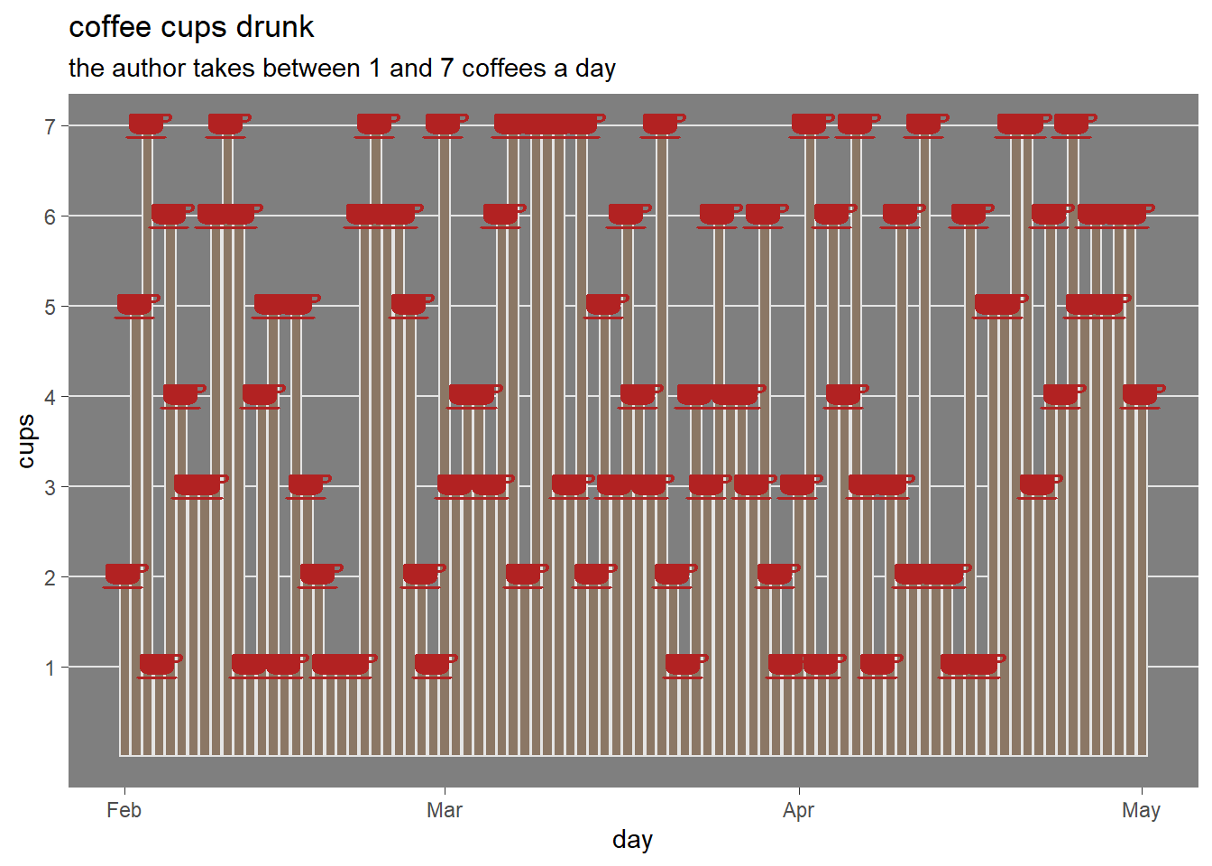
In probability theory and statistics, the Poisson distribution is a discrete probability distribution that expresses the probability of a given number of events occurring in a fixed interval of time if these events occur with a known constant mean rate and independently of the time since the last event. \[cups \sim Poisson(4)\]
In order to understand what is the meaning of the probabilistic definition, a realization from the poisson distribution, a draw from a poisson distribution with rate 4 each day, is displayed in the following graph covering last 3 months.
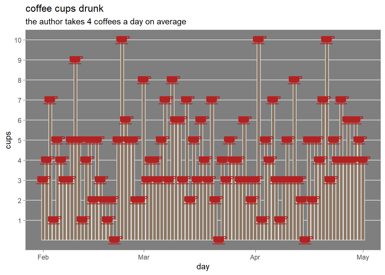
The above visualization of the poisson description of the coffee drinking habit shows how data points (cups) are more dense in the middle but also that some day cups drunk are too many.
Is this simulated coffee cups drunk visualization closer to reality?
actual data
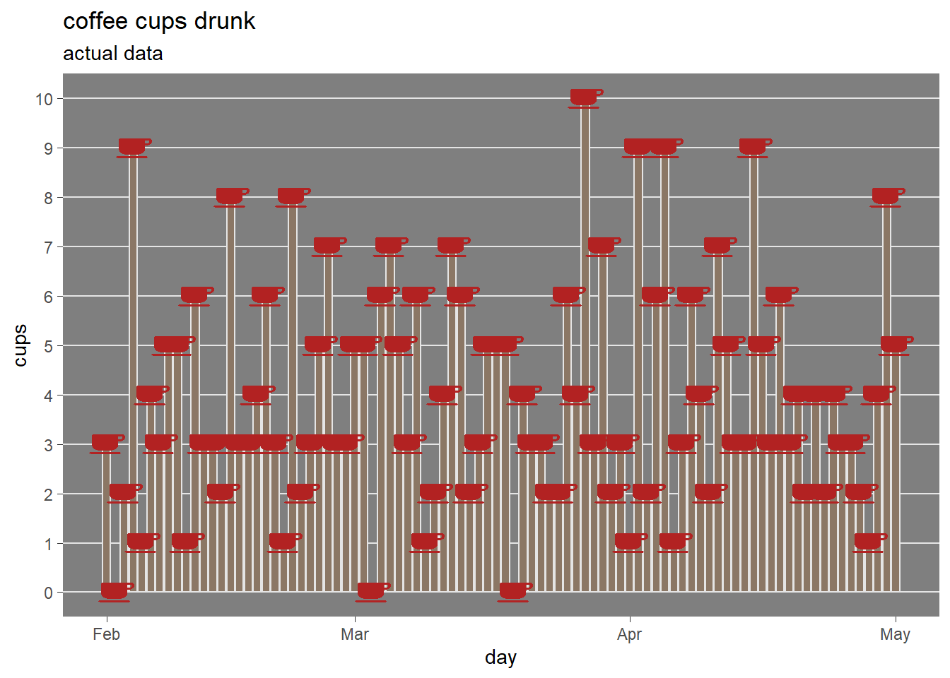
Suppose the author collected data in order to study his coffee drinking habit. Each day in the last 3 months the coffee cups drunk have been reported together with the hours worked.
The actual cups of coffee drunk each day are visualized below.
and the actual coffee cups distribution in the following graph.
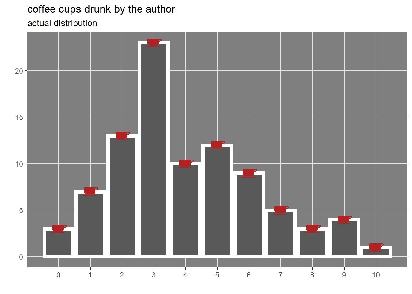
Drinking more than 6 cups of coffee each day is rare, most of the time the author drank between 2 and 6 cups.
The hypothesis that the drinking habit could be related to worked hours is supported by the following exploratory visualization in which a linear model line is fitted to the data.
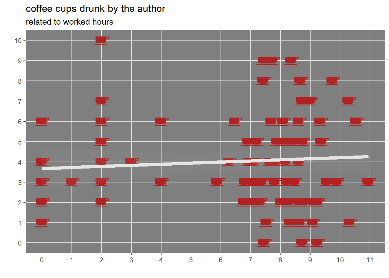 It seems that a weak positive relation exists such that number of coffee cups drunk increases as the daily working hours grow.
Another potential effect could be related also to the day of the week.
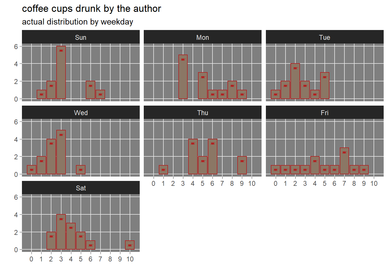
The above visualization says that coffee cups distribution changes depending on the day of week: during the weekend the coffee “drinking habit addiction” seems to be weaker. But it is likely that the relationship among the variables are as per the following directed acyclic graph (DAG).
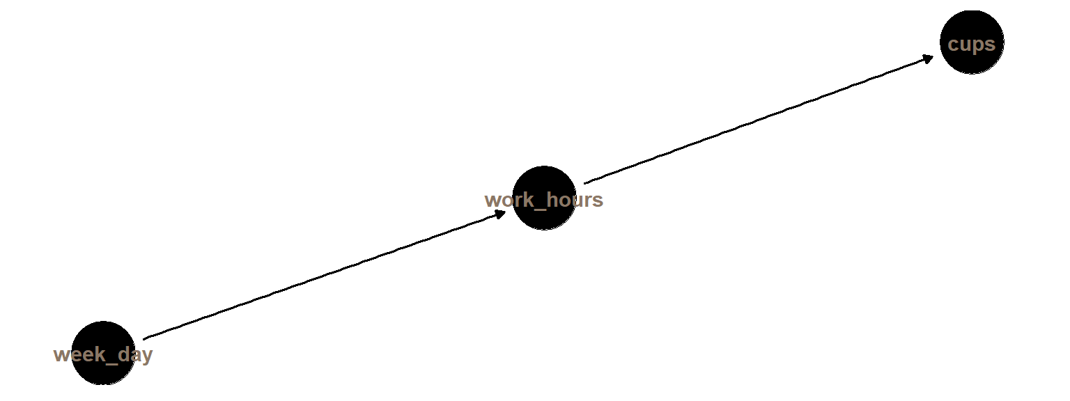
Coffee consumption (cups) depends solely on worked hours that in turn is affected by the day of the week.
a Bayesian modeling attempt
For the purpose of this post the coffee cups distribution is modeled with a simple poisson regression with the mean rate parameter (\(\lambda\)) depending only from the hours worked.
\[cups \sim Poisson(\lambda) \\ \lambda = \beta \cdot hours_{worked} \\ \beta_{prior} \sim N(0.25, 0.1)\] (A better model could include an intercept term but, for the purpose of this post, the focus is on the hours worked as the actionable variable).
The following graphs display the coefficients credible intervals and their mcmc trace.
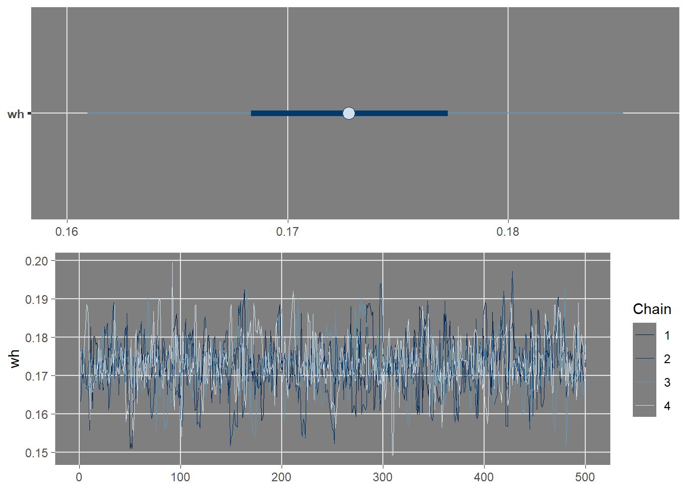
The credible interval for the worked hours beta does not contain zero. Furthermore the corresponding trace plot for the coefficient, showing the sampled values per chain and parameter throughout iterations, indicates that chains reached convergence and are well mixed together.
As a measure of the goodness of fit of this model a posterior predictive check is performed. This model validation procedure compares what the model predicts versus what it is expected (i.e. the data you have). The assumption underlying this concept is that a good model should generate fake data that is similar to the actual data set used to make the model while a bad model will generate data that is in some way fundamentally or systematically different.
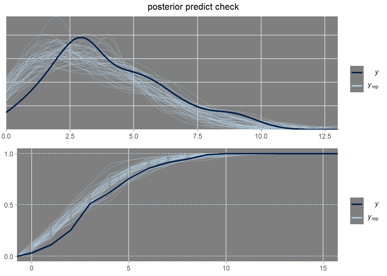
From the two plots above (first one for density overlay, the second one for the empirical cumulative distribution overlay) it is possible to state that the actual data could come form the data generating process expressed by the model especially when more than 2 cups of coffee have been drunk.
coffee related wellness
Each daily cup of coffee make the author feel better in the short term but at the end of the day if cups of coffee drunk are equal or more than 5 overall wellness decrease.
In order to proceed in this quantitative analysis a mapping from the cups of coffee drunk to a number that represent the author coffee related wellness \(wellness_{coffeee} = f(cups_{coffee})\) is defined as per the following table.
| cups of coffee | 0 | 1 | 2 | 3,4 | 5 | 6,7 | 8 | 9 | 10 |
|---|---|---|---|---|---|---|---|---|---|
| related wellness | 0 | 1 | 2 | 3 | 0 | -1 | -3 | -4 | -5 |
This coffee related wellness mapping is quite subjective but it represents the actual sensation elicited in the author itself. In other words no one can judge a feeling such as wellness if not the person who feels that sensation.
The overall daily actual coffee related wellness can be visualized below
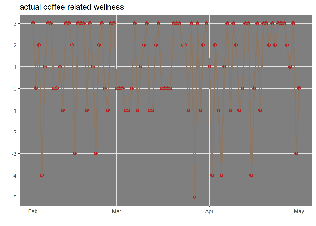
The daily mean quantified wellness related to author coffee drinking habit in last 3 months has been 0.98. Not a great but positive satisfactory number.
working hours policies
Assuming the author has to work at least 40 hours to earn a living, possible working time policies are limited to the following:
no overtime, no working weekend (form Monday to Sunday the working hours sequence is 8,8,8,8,8,0,0)
reduced working hours but working weekend (form Monday to Sunday the working hours sequence is 7,7,7,7,6,4,2)
increased working hours but Friday off (form Monday to Sunday the working hours sequence is 10,10,10,10,0,0,0)
Using the model trained for predicting the response variable (posterior distribution using Bayesian term) on this three different working hours policies, it is possible to determine the overall average coffee related satisfaction for each of them.
The computation steps involve the following two sequential mapping:
\[hours_{worked} \mapsto cups_{coffee} \mapsto wellness\]
where
- the first mapping is done applying the simple fitted Bayesian model to predict the coffee consumption;
- the second mapping is performed with the defined above mapping function that relates coffee drinking to the subjective wellness of the author.
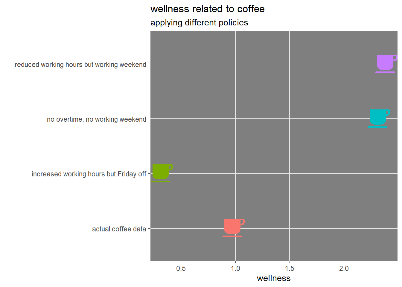
The Bayesian decision analysis on the habit of coffee consumption leads the author to recommend himself distributing working hours even during weekends by reducing the time devoted to work each working day. Compressing work in fewer days but limiting to 40 hours seems instead to lead also to a more unsatisfactory coffee drinking habit. As far as coffee drinking satisfaction is concerned, the author should in any case reduce the overall working hours and distribute them evenly.
final considerations
Although the use case analyzed is quite simple and trivial, the author’s intention is to outline an approach for probabilistic thinking.
This approach includes the following steps:
evaluate how the uncertainty related to the context of the problem is described by the subject matter expert in his or her informal language;
collect and explore data for the problem at hand;
model the uncertainty relating the response to a variable which is actionable;
map the response to a measure of (dis)satisfaction;
define the available policies on the actionable variable;
use the model to predict the measure of satisfaction for each policy and define which policy is best for the specified objective.
Bayesian decision analysis is extensively covered in literature, but not often used in public policy or business strategy context. Application to daily life decision making seems to be really rare.
The author believes that the ultimate goal of the data science cultural shift is to promote probabilistic thinking as an effective counterpart to any form of reasoning that mainly implies the principle: go where your heart takes you.
Feel free to email me if you would like to go deeper in the analysis, thanks for reading!
The analysis shown in this post have been executed using R as main computation tool together with its gorgeous ecosystem ( tidyverse included). In particular Bayesian analysis was based on rstanarm and bayesplot packages.