
Public debate in Italy about how the country fit into Euro zone economy is always active. It is one of the topic which divides Italian political parties the most. In order to help forming informed opinion this post delve into analysis of Gross Domestic Product macroeconomic data only. The analysis in this post provides a limited but insightful view on the issue.
analysis outline
After a brief introduction to macro economic data under study, the analysis in this post considers the time series levels and the growths or rate of change of Gross Domestic Product for Italy and Euro Area performing a rough comparison.
In particular analysis of gross domestic product levels is articulated in:
visualization and comparison of Italy and Euro Area time series;
decomposition of levels in trend and in cycle part for both the time series.
The comparative analysis of gross domestic product growths includes:
assessment of time series stationarity;
growths distribution statistical analysis;
check of dependence of Italy growth from Euro Area growth using a minimal Vector Auto Regression model;
forecasting of growth as no COVID-19 pandemic occurred.
Gross Domestic Pruduct: Eurozone vs. Italy
The Organization for Economic Co-operation and Development (OECD) defines Gross Domestic Product (GDP) as “an aggregate measure of production equal to the sum of the gross values added of all resident and institutional units engaged in production and services (plus any taxes, and minus any subsidies, on products not included in the value of their outputs).”
Comparing GDP of Italy with the overall Euro area GDP could help in get some insights about our primary question: how Italian economy fits in that of Euro Area.
Euro area, or euro zone, i.e. where Euro is the official currency, includes 19 countries: Austria, Belgium, Cyprus, Estonia, Finland, France, Germany, Greece, Ireland, Italy, Latvia, Lithuania, Luxembourg, Malta, the Netherlands, Portugal, Slovakia, Slovenia and Spain.
The following time series are used in the proceeding of this post:
Real Gross Domestic Product (Euro/ECU series) for Euro Area;
Real Gross Domestic Product for Italy.
Both the GDPs are “real” i.e. normalized by the Consumer Price Index (CPI). CPI is a measure that examines the weighted average of prices of a basket of consumer goods and services, such as transportation, food, and medical care. Changes in the CPI are used to assess price changes associated with the cost of living.
Both the GDP time series are quarterly in frequence and already seasonally adjusted.
Original data are measured in millions of Euros.
Source of the data is Eurostat, the statistical office of the European Union. Data have been retrieved from FRED on July 2020.
GDP levels
To get a grasp of what has happened in last 20 years, Euro Area (EA) and Italy (IT) GDP levels have been visualized towards time.
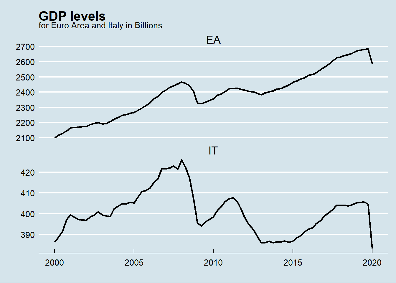
The graph highlights big difference in the trend. Euro Area GDP shows a constant upward trend except for the world financial crisis in 2008. Italian GDP has a more complex path with extended crisis periods. The impact of international financial crisis in 2008 followed by the national debt crisis in 2011 is clearly visible.
It is also possible to visualize Italy contribution to Euro area GDP throughout almost 20 years.
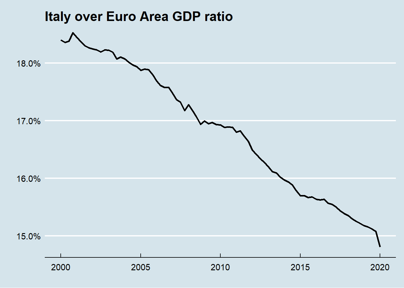 In twenty years Italy lost more then 3% of his contribution to Euro Area GDP. Furthermore it is noticeable that Italy contribution to GDP trend is continuously downward.
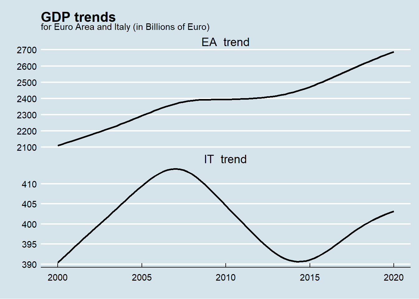
Italy and Euro Area GDP trend
In order to understand better where the differences between Italy GDP and Euro Area one are, the two time series has been decomposed in their trend and cyclic part using a Hodrick-Prescott filter. The Hodrick-Prescott filter is used in macroeconomics, especially in real business cycle theory, to remove the cyclical component of a time series from raw data.
The trend part visualized below shows a significant difference in trend from 2008 onward. While Euro Area GDP maintains his upward trend. Italy GDP dropped till 2015 and then it went up without reaching the level before 2008 (not considering COVID-19 crisis).
GDP business cycles
The cyclic part of the time series highlights the overall economic cycle to which Europe has been subject to.
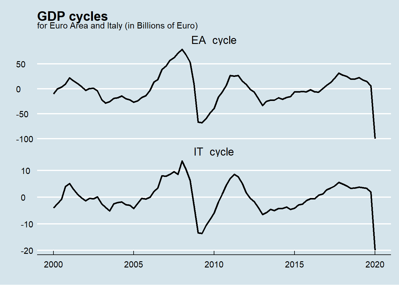 Again the global financial crisis (2008), the national debt crisis (2011) and the COVID-19 one (2020) are clearly visible.
The business cycles of Euro Area and Italy are really similar. In statistics this is said that they are highly correlated.
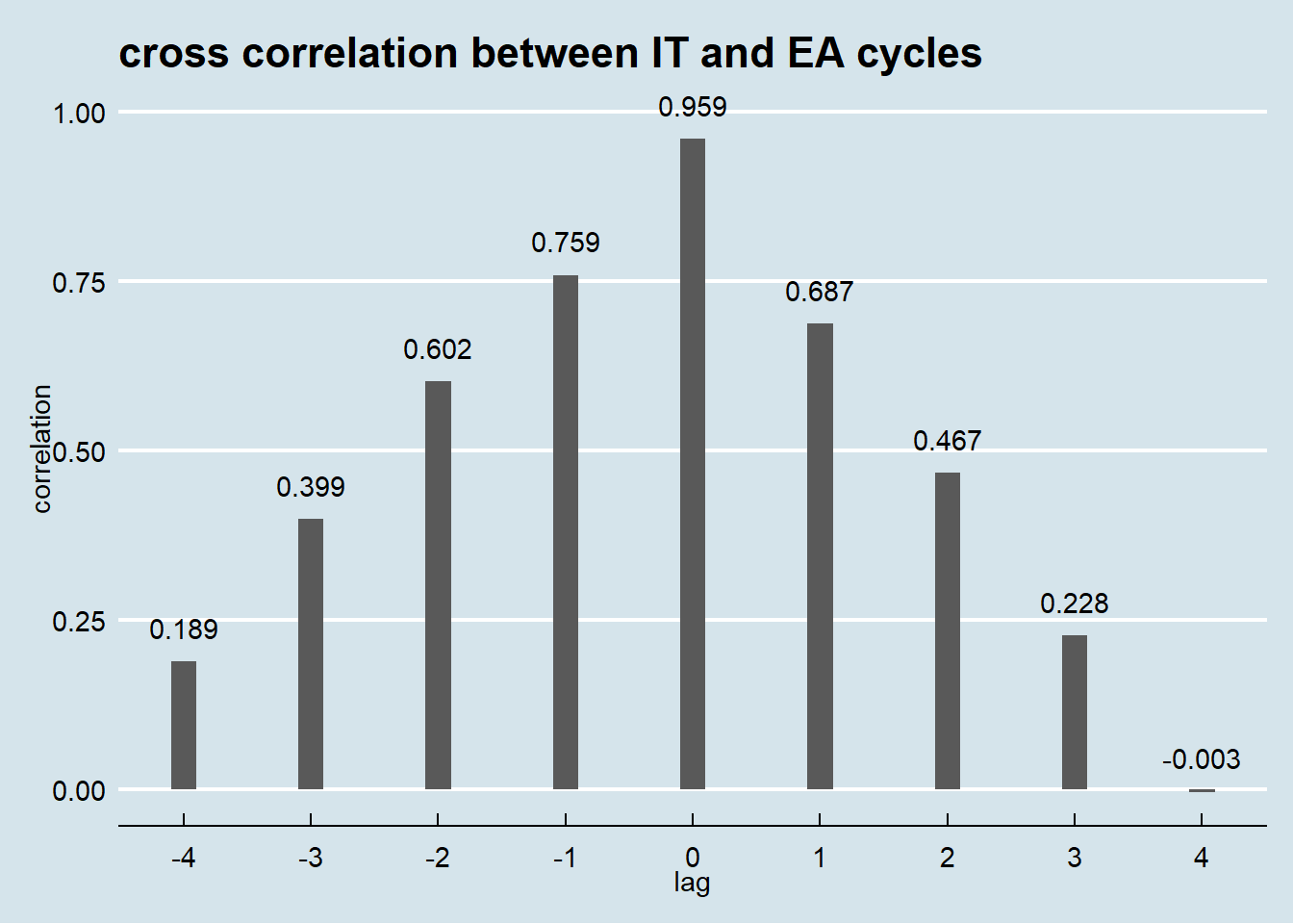
The plot above, outcome of cross correlation analysis, identifies lags of the Italy GDP cycle that might be useful predictors of Euro Area business cycle at time t. With no lag the two series are almost collinear.
GDPs growth
The gross domestic product growth rate measures how fast economy is growing (or shrinking). GDP growth rate is therefore a vital indicator of economic health.
In order to proceed with the analysis, GDP growth rates has been computed as the rate of change for Italy GDP quarterly data and for a fictitious Euro Area of 18 country (without Italy) (EA18) pretending to separate Italy from Euro Area.
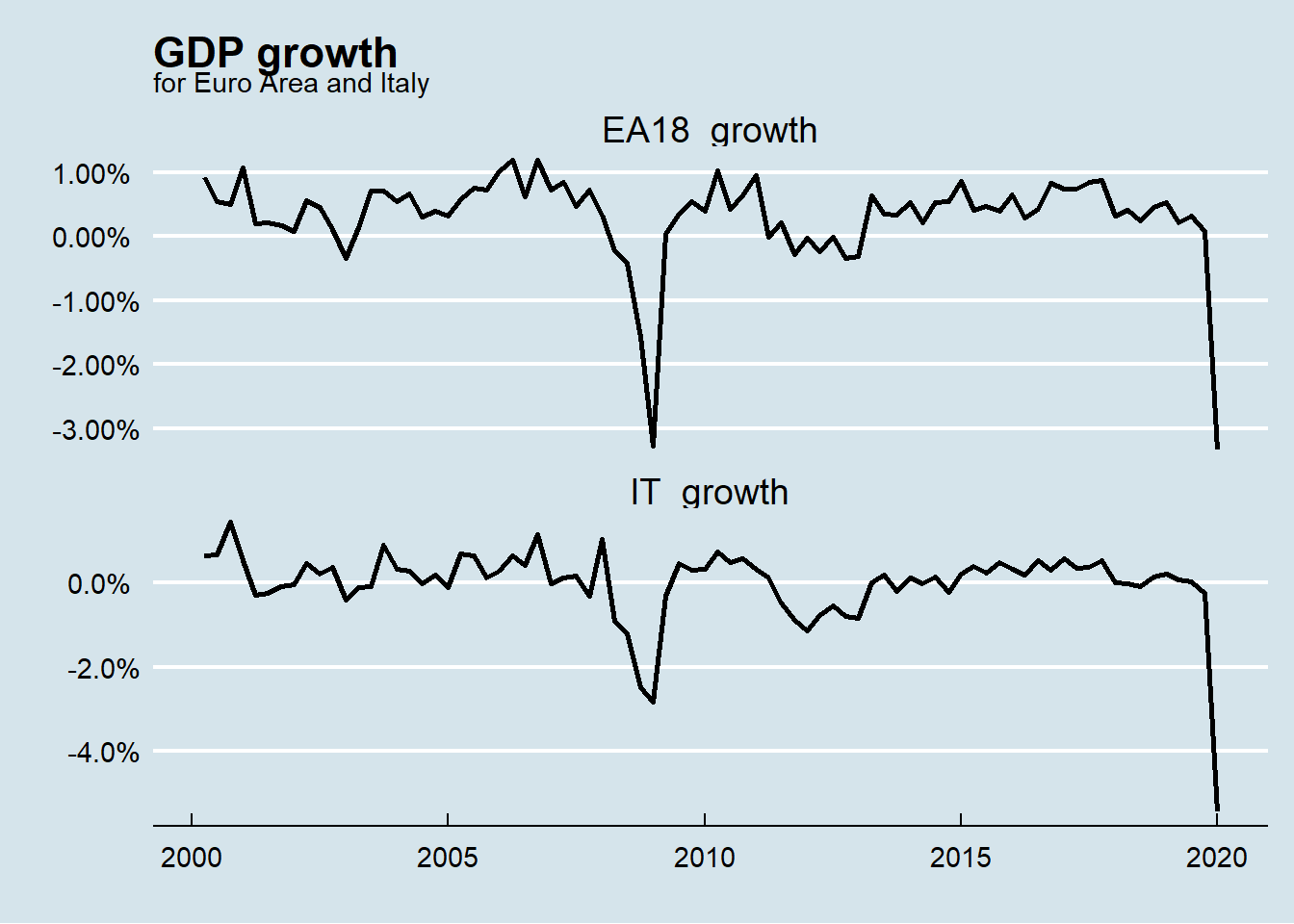
GDP growths are visualized below (note the difference in y scale) and remember that the number reported are quarterly data not annualized.
stationarity
One of the most important characteristic for time series to be modeled is their stationarity. A time series is said to be weakly stationary when it has constant mean and variance throughout the time.
The two time series under study seems not to be exactly weakly stationary as confirmed by the Philips-Perron test. This statistical test checks the null hypothesis that a unit root is present in a time series against the alternative that the series is stationary.
##
##  Phillips-Perron Unit Root Test
##
## data:  gdps_growth$IT_growth
## Dickey-Fuller = -2.8008, Truncation lag parameter = 3, p-value = 0.248
##
## Phillips-Perron Unit Root Test
##
## data: gdps_growth$EA18_growth
## Dickey-Fuller = -3.5242, Truncation lag parameter = 3, p-value =
## 0.04539Reported p-values higher than 5% means that the null hypothesis of presence of a unit root cannot be rejected.
Getting rid of the last GDP quarter referring to COVID-19 crisis that is indeed a clear outlier, the time series become weakly stationary as confirmed by Philips-Perron test.
##
##  Phillips-Perron Unit Root Test
##
## data:  gdps_growth_st$IT_growth
## Dickey-Fuller = -4.3275, Truncation lag parameter = 3, p-value = 0.01
##
## Phillips-Perron Unit Root Test
##
## data: gdps_growth_st$EA18_growth
## Dickey-Fuller = -4.7402, Truncation lag parameter = 3, p-value = 0.01Without 2020 the p-values are below 5% so the null can be rejected.
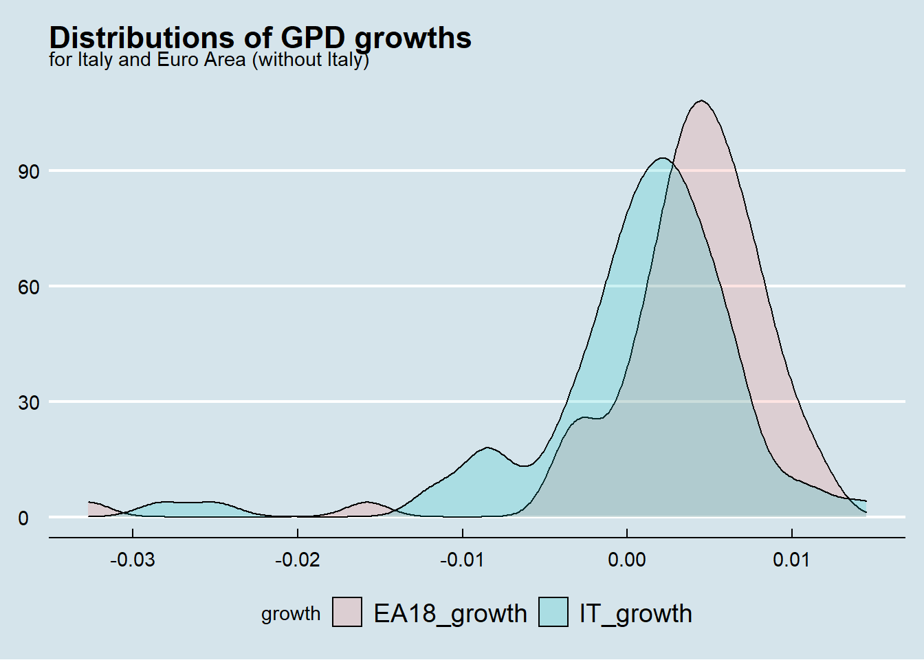
GDP growths distributions and statistics
The following plot compares the distributions of Italy growth towards de-Italianized Euro Area.
| Italy | Euro Area 18 | |
|---|---|---|
| mean | 0.00059 | 0.00361 |
| standard deviation | 0.00661 | 0.00594 |
| skewness | -1.82036 | -3.33027 |
| kurtosis | 5.79503 | 17.06136 |
where such measures describe the probability distribution
mean represents the average value for growth. Quarterly growth for Italy is 0.05 %, the figure for Euro Area without Italy is 6 times higher;
standard deviation measures the amount of variation or dispersion of the growths values. Italy growth seems to be slightly more variable than Euro Area (18 country) one;
skewness measures asymmetry in the distribution. Both distribution appears distorted or skewed to the left (towards low and negative value);
kurtosis measures the “tailedness” of the distributions. Both distributions have more observations in tails than in a normal distribution (kurtosis = 3) with Euro Area distribution deviating significantly from normal.
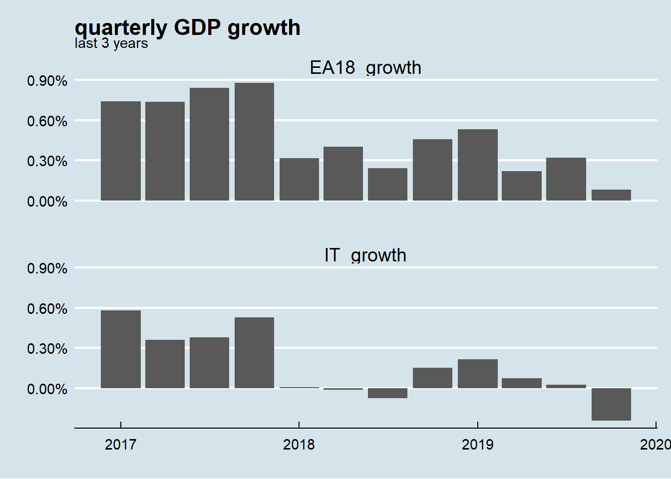
last three years of GDP growth
In order to get a closer look at GDP growths the following plot visualizes the last 3 years (from 2017 to 2019).
| year | Italy | Euro_Area |
|---|---|---|
| 2017 | 1.7 | 2.54 |
| 2018 | 0.8 | 1.91 |
| 2019 | 0.3 | 1.23 |
vector autoregression
Starting from the hypothesis that GDP growth for Italy and for Euro Area not including Italy are somewhat interdipendent affecting each other intertemporally, the 2 GDP growth series can be modeled using vector autoregression (VAR). VAR models generalize the univariate autoregressive model (AR model) by allowing for more than one evolving variable. All variables in a VAR enter the model in the same way: each variable has an equation explaining its evolution based on its own lagged values, the lagged values of the other model variables, and an error term.
Properties of the VAR model are usually summarized using impulse response analysis which main purpose is to describe the evolution of a model’s variables in reaction to a shock in one or more variables.
For our analysis purpose it is interesting to see how Italian GDP growth could react to a positive impulse in fictitious Euro Area at 18 country economy growth.
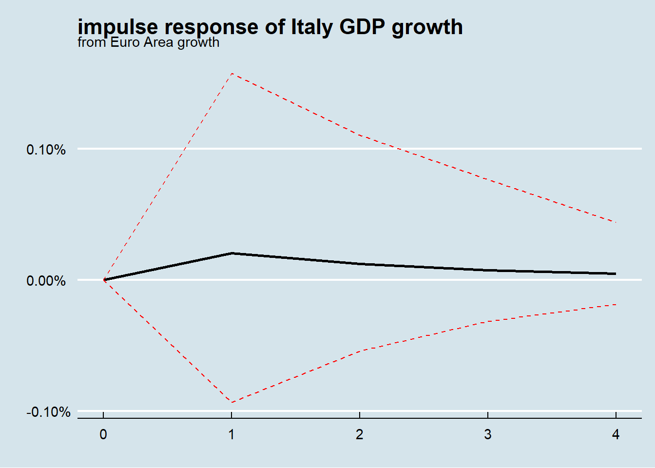
The interpretation of graph above is straightforward: an impulse (shock) to Euro Area at 18 country growth at time zero has small effect the next period and the effect become smaller and smaller as the time passes. The dotted lines show the 95 percent interval estimates of these effects that are clearly not statistically significant.
The variance decomposition indicates the amount of information each variable contributes to the other variables in the auto regression. It determines how much of the forecast error variance of each of the variables can be explained by exogenous shocks to the other variables.
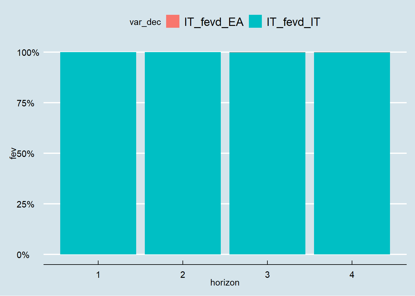
The graph above shows that almost 100 percent of the variance in Italian GDP growth is caused by the Italian GDP growth itself despite the exogenous shock to Euro Area not including Italy.
| horizon | Italy | Euro Area 18 |
|---|---|---|
| 1 | 1.00000 | 0.00000 |
| 2 | 0.99891 | 0.00109 |
| 3 | 0.99867 | 0.00133 |
| 4 | 0.99859 | 0.00141 |
Granger causality
The Granger causality test is a statistical hypothesis test for determining whether one time series is useful in forecasting another. In this case the Granger causality test evaluates if Euro Area growth lagged values provide statistically significant information about future values of Italy GDP growth.
## $Granger
##
##  Granger causality H0: EA18_growth do not Granger-cause IT_growth
##
## data:  VAR object var_mdl
## F-Test = 0.12253, df1 = 1, df2 = 150, p-value = 0.7268
##
##
## $Instant
##
##  H0: No instantaneous causality between: EA18_growth and IT_growth
##
## data:  VAR object var_mdl
## Chi-squared = 27.807, df = 1, p-value = 1.34e-07
The test result states with a high p-value that Euro Area growth (without Italy) do not Granger-cause Italy GDP growth .
forecasting Italy GDP growth (no COVID-19 crisis)
In order to predict future points in the Italy GDP growth series (forecasting), an ARIMA model could be fitted to data.
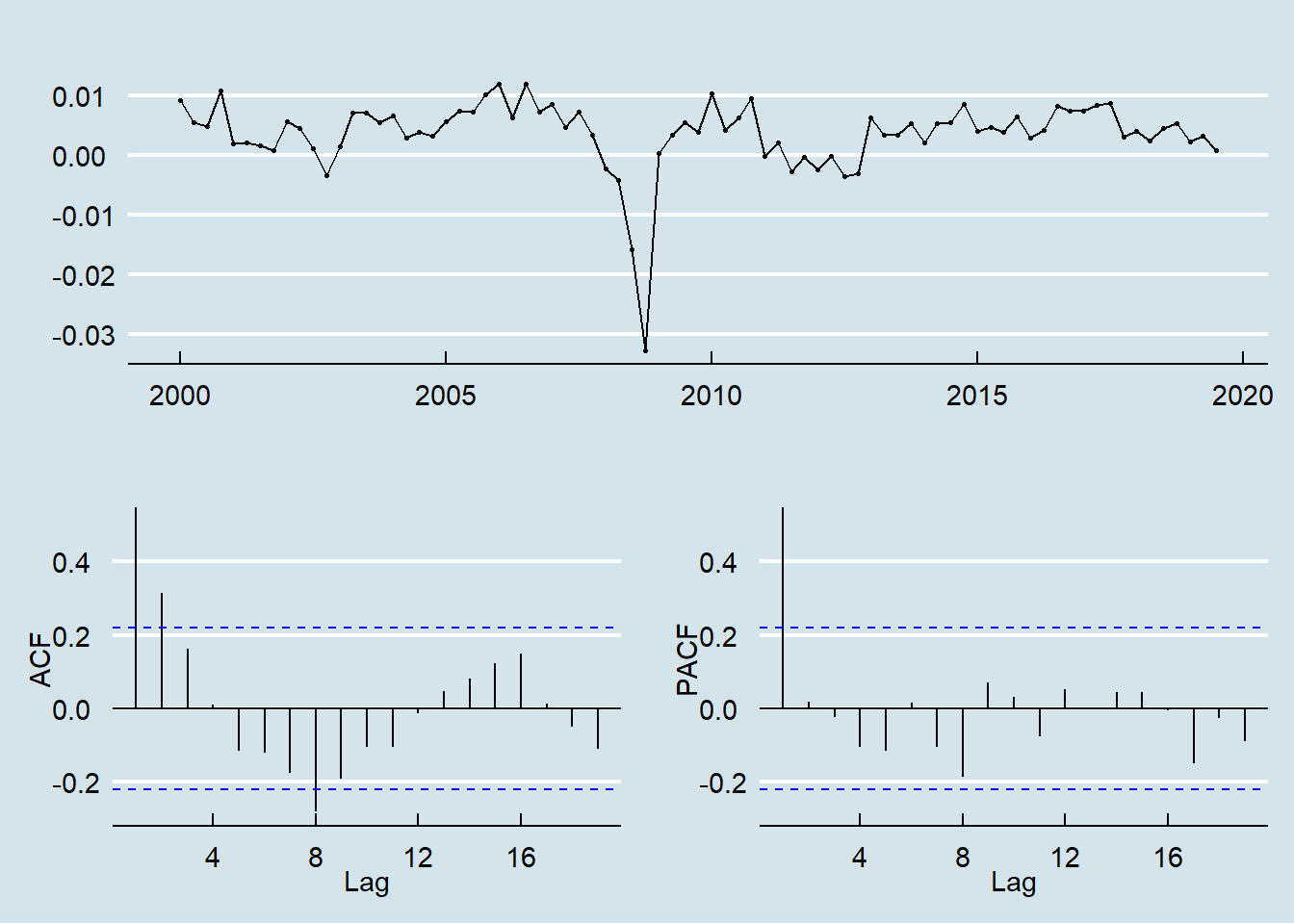
Analyzing the series and the auto correlation and partial auto correlation plot it is possible to identify the model specification.
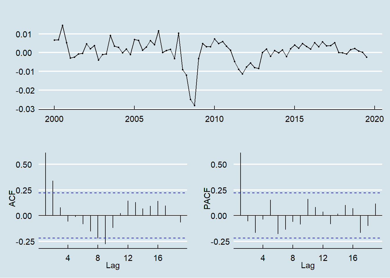 The PACF shows a single spike at the first lag and the ACF shows a tapering pattern therefore an AR(1) model is indicated.
| term | estimate | std.error |
|---|---|---|
| ar1 | 0.61279 | 0.08792 |
| intercept | 0.00064 | 0.00148 |
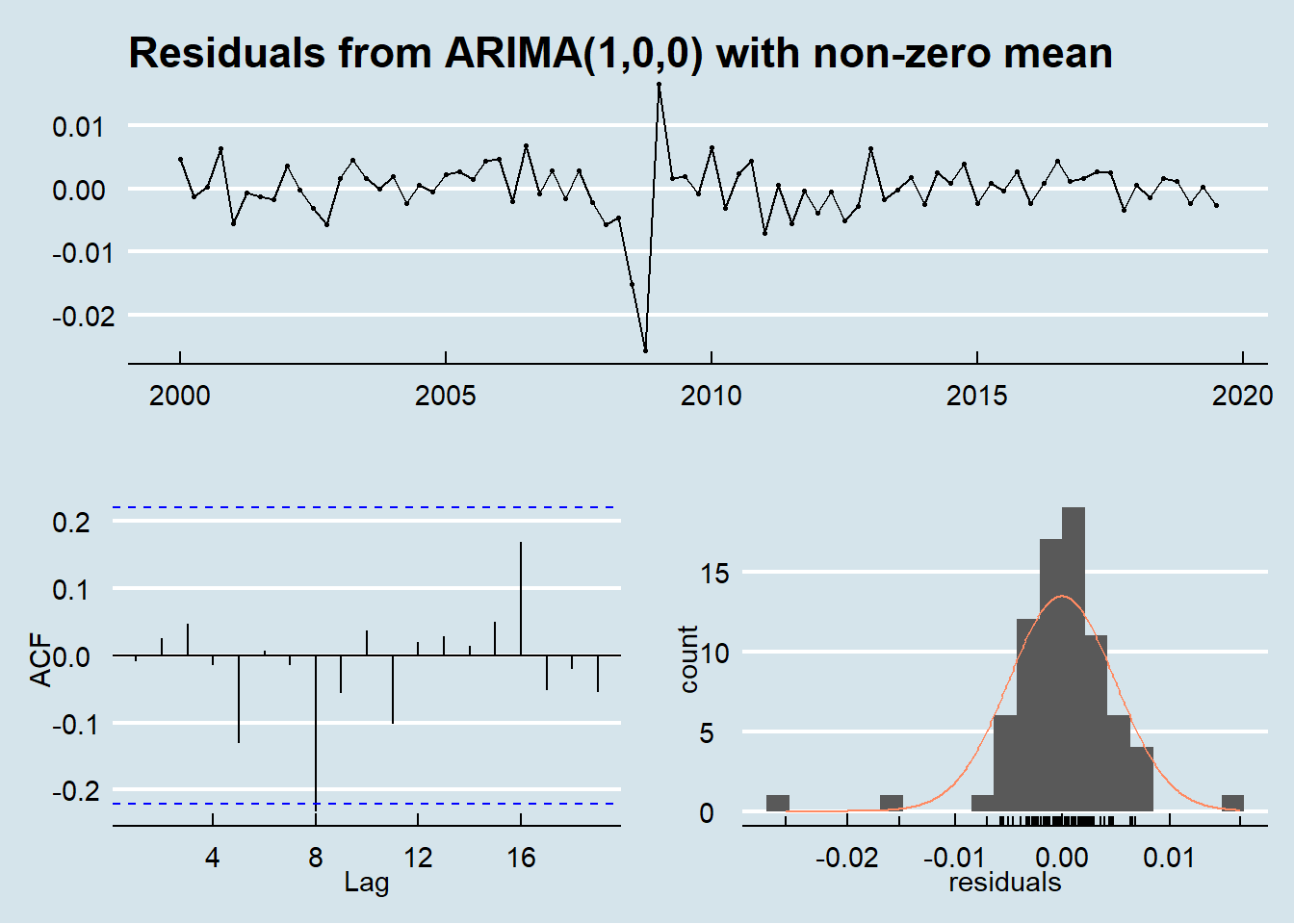
In order to assess the goodness of fit of the AR(1) model, the residuals against time, their autocorrelation and their distribution have been plotted.
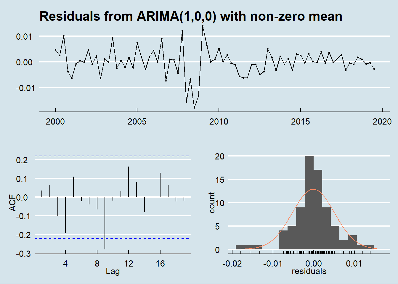 The ACF of the residuals show non-significant values at all lags except for a barely significant residual auto correlation at lag 9.
Furthermore the residuals show a almost normal distribution.
This confirm the goodness of the fit of the AR(1) model for the Italian GDP growth series.
The ACF of the residuals show non-significant values at all lags except for a barely significant residual auto correlation at lag 9.
Furthermore the residuals show a almost normal distribution.
This confirm the goodness of the fit of the AR(1) model for the Italian GDP growth series.
It is now possible to forecast growth one year ahead (4 quarters horizon)
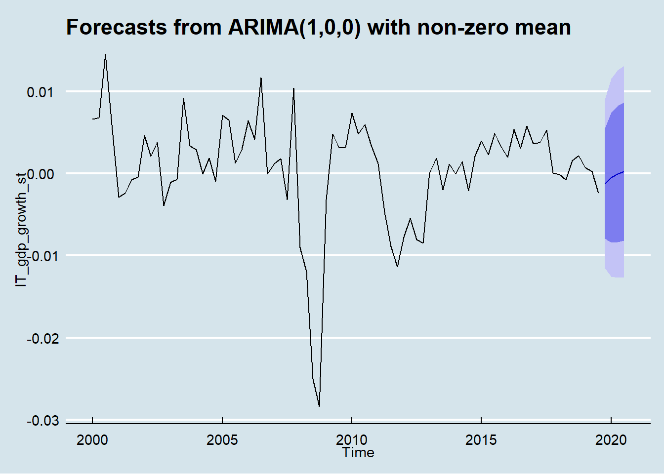 If no COVID-19 pandemic occurred Italy GDP growth will likely recover a bit from a slightly negative value.
forecasting Euro Area GDP growth (no COVID-19 crisis)
Series against time, auto correlation and partial auto correlation plots for Euro Area GDP growth are shown below.
 The PACF shows a single spike at the first lag and the ACF shows a tapering pattern: also in this case an AR(1) model is indicated.
The fitted auto regressive model of order 1 has the following parameters:
| term | estimate | std.error |
|---|---|---|
| ar1 | 0.54822 | 0.09340 |
| intercept | 0.00365 | 0.00121 |
In order to assess the goodness of fit of the AR(1) model, the residuals against time, their autocorrelation and their distribution have been plotted.
 The residuals show a almost normal distribution and the ACF of the residuals shows non-significant values at all lags except for a barely significant residual autocorrelation at lag 8 thus confirming the goodness of the fit of the AR(1) model.
It is now possible to forecast growth one year ahead (4 quarters horizon) using the fitted model.
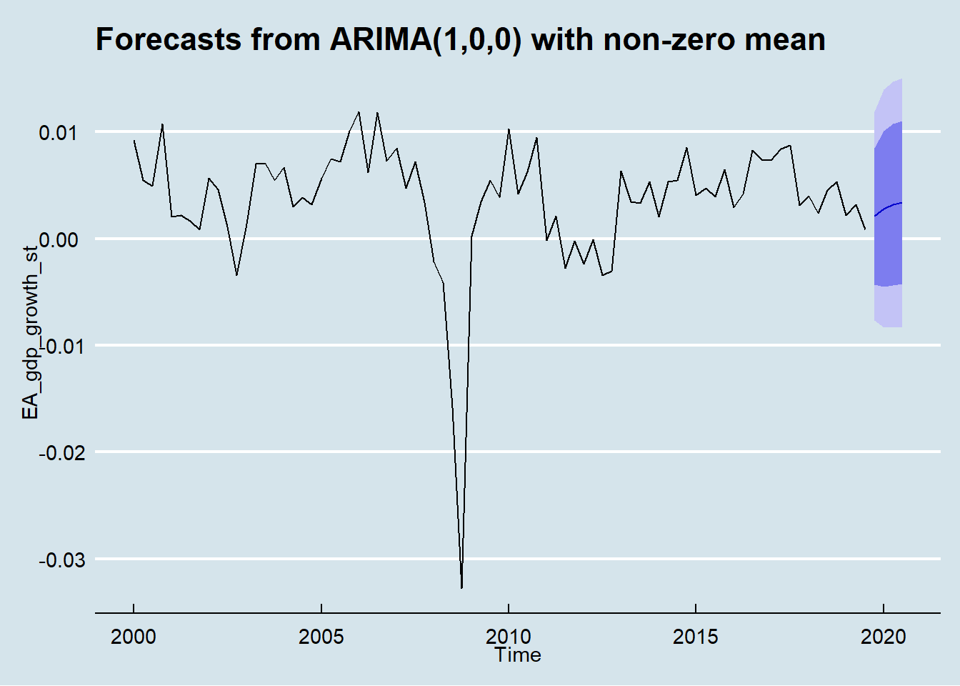 If no COVID-19 crisis will occur, the Euro Area GDP without growth, not including Italy contribution, would have slightly raise but not reaching values of previous year.
findings
This post performed a quick and dirty time series analysis applied to macro economic data (and not a macro economic analysis for which the Author is not qualified). Nonetheless the findings of the analysis have the force of facts.
And the main facts are:
in about 20 years Italy lost about 3% of GDP contribution to Euro Area GDP;
Euro Area and Italy are subject to the same business cycle;
Italy showed a significantly different economical trend from Euro Area;
Italy growth average value is about 6 times lower than Euro Area growth mean considering last 20 years;
Euro Area GDP growth positive shock shouldn’t impact significantly on Italy growth as suggested by a VAR model;
if no COVID-19 crisis occurred (GDP quarterly figures for the first quarter 2020 are outliers in respect of the time series)… forecasts based on auto regressive models showed that GDP growth would have slightly improved both for Italy and for Euro Area but Italy would not have filled the gap.
These numerical facts, together with many others data analysis outcomes, should be part of the public discussion on how Italy fit into Euro Zone economy helping in separating narratives about Euro Area from reality. The Author believes that the responsibility for interpretation is up to the informed reader. Data science role is enabling the formation of opinions based on sounding data analysis.
Feel free to email me if you would like to delve into analysis details, thanks for reading!
The analysis and forecasts shown in this post have been executed using R as main computation tool together with its gorgeous ecosystem. In particular vector autoregression relied on “vars” package while forecasting relied on “forecast” package.