
Serie A football season 2019-20 stopped in March due to covid-19 pandemic. Even if the championship just re-started in late June, it is likely it will be a different competition history because of teams shape changes after almost 4 months of inactivity. Therefore, as an exciting sport analytics exercise, this post predicts and simulates the final results of Serie A 2019-20 season on the basis of already played matches results without considering the occurred interruption.
Serie A till March 2020
Serie A is regarded as one of the best football leagues in the world and it is often depicted as the most tactical national league. During the season, which usually runs from August to May, each club plays each of the other teams twice; once at home and once away, totaling 38 games for each team by the end of the season. Thus, in Italian football a true round-robin format is used. In the first half of the season, called the andata, each team plays once against each league opponent, for a total of 19 games. In the second half of the season, called the ritorno, the teams play in exactly the same order that they did in the first half of the season, the only difference being that home and away situations are switched. In this year, due to covid-19 pandemic, Serie A competition stopped at 26th round, the seventh round of ritorno with 4 matches in 25th round to be recovered too.
the data
Match scores data for Serie A season 2019-20 have been downloaded from site http://www.football-data.co.uk/data.php
Serie A standings at championship stop
Going back to March 9, when the last match before the stop was played, the standings were as visualized in the following infographic.
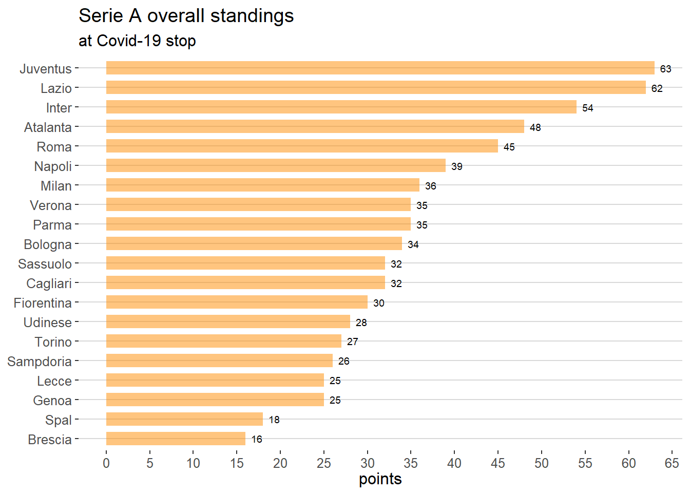 At the top of standings Juventus was ahead of Lazio by only 1 point with all the other clubs far away.
At the bottom Brescia and Spal were respectively 9 and 7 points from the third to last.
At the top of standings Juventus was ahead of Lazio by only 1 point with all the other clubs far away.
At the bottom Brescia and Spal were respectively 9 and 7 points from the third to last.
predicting season final results
In order to answer the intriguing question, at least for Italian football fans and the Author alike, about the final Serie A ranking (without covid-19 pandemic), three quantitative analysis have been exploited:
pythagorean win expectations;
Davidson model of competition;
Monte Carlo simulation drawing from Poisson distributions of goals scored.
pythagorean win expectation
Stealing from sabermetrics the pythagorean win expectation method, it is possible to estimate the number of points a given club would have won completing Serie A 2019-20 competition. Compared to the original idea, it is needed to take into account the result of the tie which is not an actual possibility in baseball.
Therefore the formula used is given by: \[ pytagoreanPoints = winExpectation * remainingMatches * avgPtsD istributed \]
where
pythagorean ‘winExpectation’ is calculated as per the following formula: \[winExpectation = \frac{GoalsScored^{exponent}}{GoalsScored^{1.32} + GoalsConceded^{exponent}}\]
remainingMatches equals 12 for every Club except Atalanta, Cagliari, Hellas Verona, Inter, Parma, Sampdoria, Sassuolo and Torino because their matches in 25th round have been postponed.
average points distributed in a match takes in consideration the potential tie result and it is calculated for all clubs as \[avgPtsD istributed = \frac{totalSeasonPoints}{matchesPlayed}\]
which result in 2.7734375 average points distributed each match.
model tuning
Even if some literature fixes the exponent for soccer, the exponent used in this analysis has been tuned using Serie A 2019-20 data only.
The tuning procedure computes pythagorean points for each club for matches played and see how good is the fit to achieved points through adjusted R squared metrics.
Adjusted R squared measures how much of the variability of the data are explained by the linear model.
The following visualization explains better than words the grid search optimization performed.
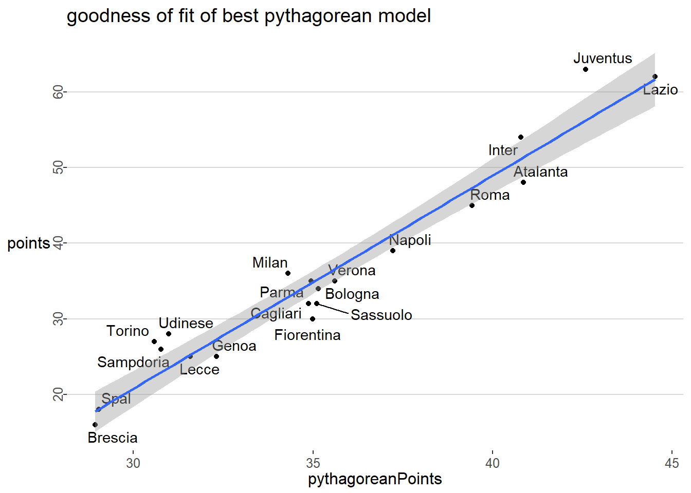
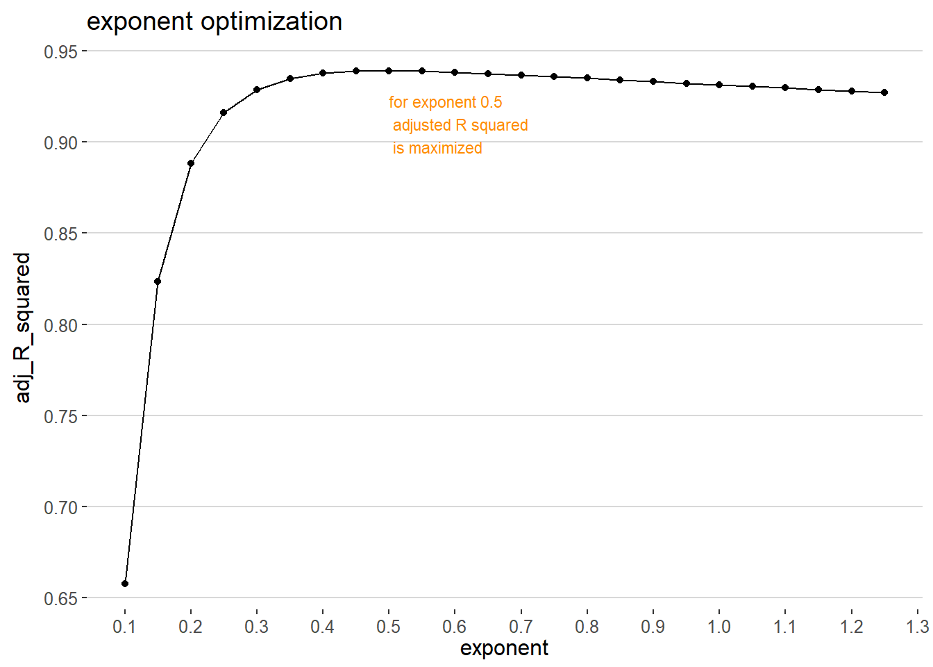 The linear model fit of points achieved vs points expected can be visualized for the best model with exponent 0.5.
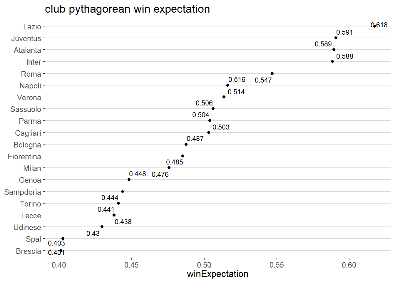
club win expectation
The win expectation for each club are shown in the following infographic.
projected final results
Applying the formula using exponent equal 0.5 to our interrupted Serie A results, the win expectation leads to the following final results.
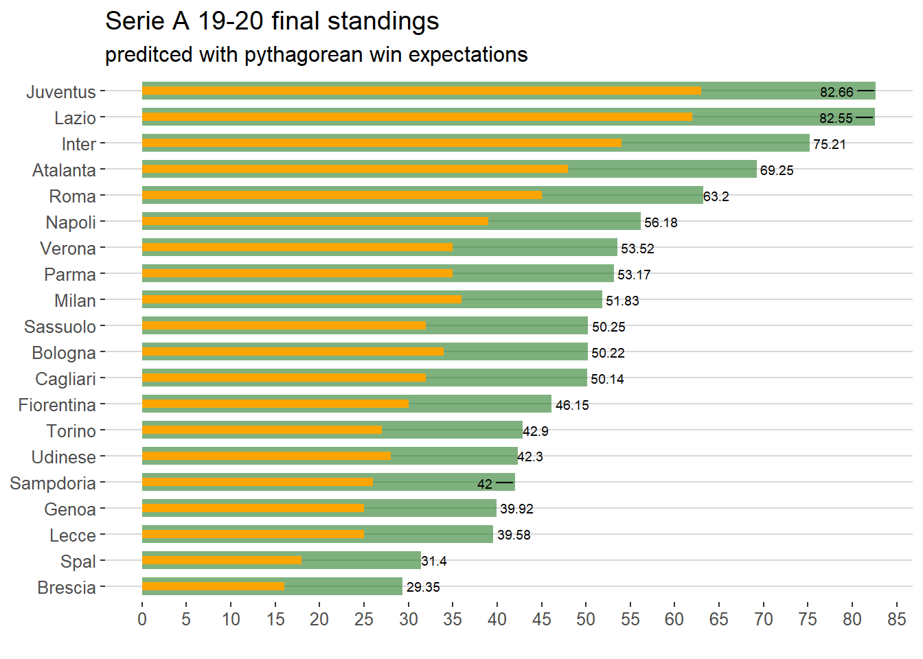
This predicted final standings are a projection of the result achieved till the championship stop. Juventus wins over Lazio for tenths of a point which is not an actual possibility in football.
The predictions obtained through pythagorean model do not take into account:
any potential dynamic of win expectation due to teams shape changes;
the remaining matches difficulties due to having already or not played with strongest clubs.
davidson model of competition
Stealing from tennis analytics, it is possible to make ranking predictions from pairwise comparison using Davidson extension to Bradley-Terry model of competition 1. Davidson model takes into account the probability of a tie and home advantage as explicit predictor. The model is fitted on few data points but the graph of comparison is fully connected because the first half of the season has been already played and therefore all teams played against everyone else.
Davidson model parameters
The Davidson model explicitly model ties but even if related coefficient is statistically significant the effect size (already transformed in response unit) is not so relevant. The home advantage predictor coefficient is not statistically significant.
| term | estimate | p.value |
|---|---|---|
| home.adv | 1.09021 | 0.60473 |
| tie.max | 0.37055 | 0.00000 |
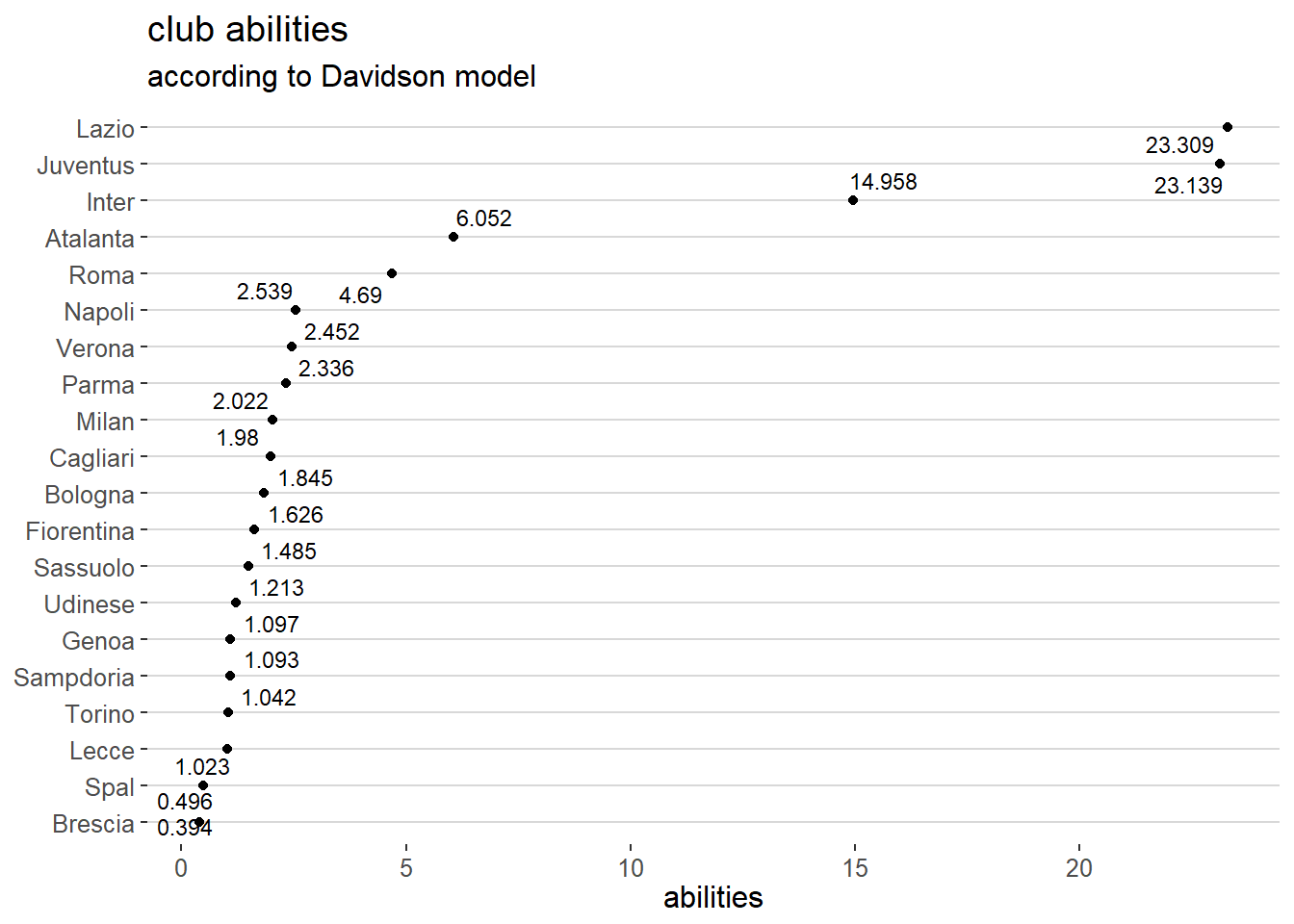
The club “abilities” found by the model are showed in the following infographic.
predicting the rest of the season
Applying the fitted Davidson model the clubs will get the following points in the remaining part of the season.| Club | matches_to_play | predicted_points |
|---|---|---|
| Atalanta | 13 | 17 |
| Bologna | 12 | 10 |
| Brescia | 12 | 6 |
| Cagliari | 13 | 11 |
| Fiorentina | 12 | 10 |
| Genoa | 12 | 10 |
| Inter | 13 | 35 |
| Juventus | 12 | 32 |
| Lazio | 12 | 32 |
| Lecce | 12 | 10 |
| Milan | 12 | 10 |
| Napoli | 12 | 12 |
| Parma | 13 | 14 |
| Roma | 12 | 15 |
| Sampdoria | 13 | 10 |
| Sassuolo | 13 | 10 |
| Spal | 12 | 8 |
| Torino | 13 | 10 |
| Udinese | 12 | 10 |
| Verona | 13 | 15 |
The related final standings are visualized below.
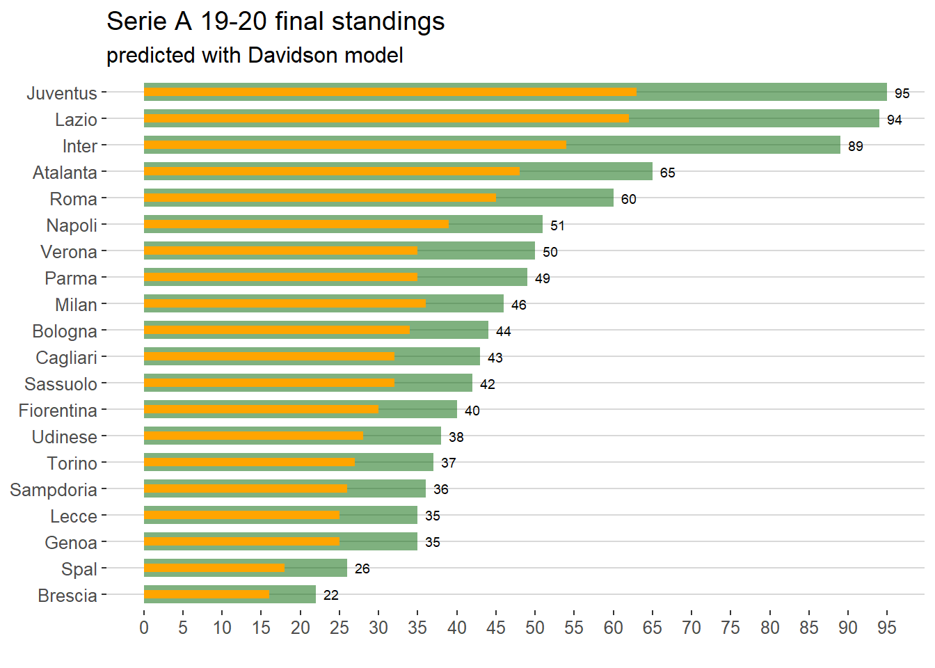
The final standings predicted by the davidson model consider each match to be played and relative abilities strength of home and away team. The result highlight the huge gap in strength among the first three teams, which will win almost all the points available, and the other teams.
Monte Carlo simulation
In this third part of the post the idea is to simulate every remaining match by running a Monte Carlo simulation drawing the results from the fitted Poisson distributions.
‘Monte Carlo simulation’ propagates uncertainties in model inputs into uncertainties in model outputs (final standings). Monte Carlo simulation relies on the process of explicitly representing uncertainties by specifying inputs as probability distributions. If the inputs describing a system are uncertain, the prediction of future performance is necessarily uncertain. That is, the result of any analysis based on inputs represented by probability distributions is itself a probability distribution.
Inputs for this simulation are goals scored and conceded in each match. The distribution this goals should follow is a Poisson distribution as per literature. The Poisson distribution is a discrete probability distribution that expresses the probability of a given number of events occurring in a fixed interval of time (a match) if these events occur with a known constant mean rate and independently of the time since the last event [wikipedia]. Its PMF is \[ p(goals = k)=\frac{\lambda^k e^{-\lambda}}{k!}\] where \(\lambda\) is both the mean and the variance of the distribution.
In order to check this is reasonably correct, the histogram for actual total goals scored in the played matched of season 2019-20 is plotted below against the Poisson distribution with lambda parameter equals the mean of total goals scored at home and away.
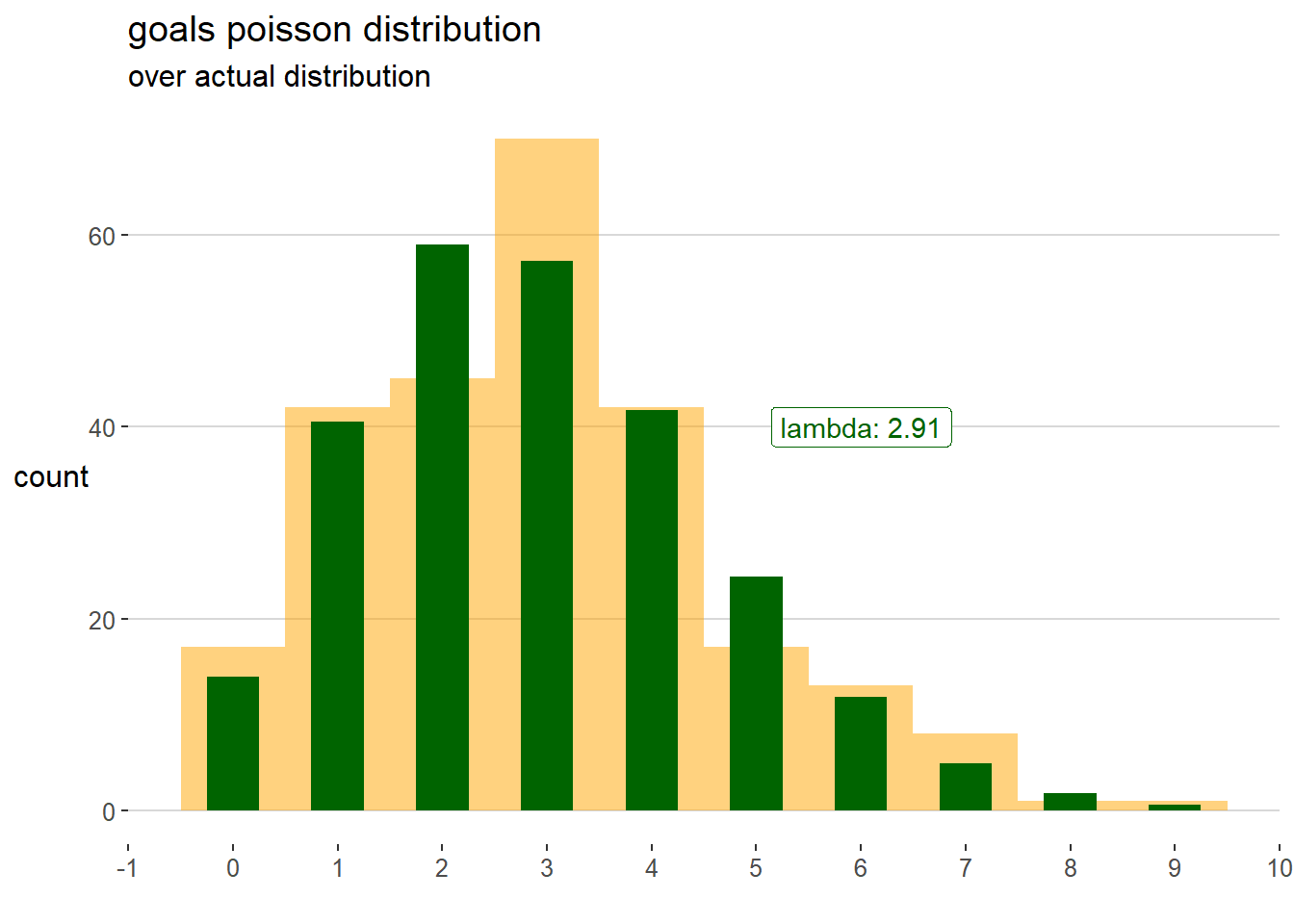
Also a formal goodness of fit test confirms that actual distribution is not significantly different from Poisson checking the old fashioned p value > 0.05.
## Chi-squared statistic:  9.790972
## Degree of freedom of the Chi-squared distribution:  5
## Chi-squared p-value:  0.08137932
## Chi-squared table:
##      obscounts theocounts
## <= 0  17.00000   13.88925
## <= 1  42.00000   40.47413
## <= 2  45.00000   58.97208
## <= 3  70.00000   57.28277
## <= 4  42.00000   41.73140
## <= 5  17.00000   24.32158
## > 5   23.00000   19.32879
##
## Goodness-of-fit criteria
##                                1-mle-pois
## Akaike's Information Criterion   995.4709
## Bayesian Information Criterion   999.0161
Same check is performed for goal scored by home and by away team
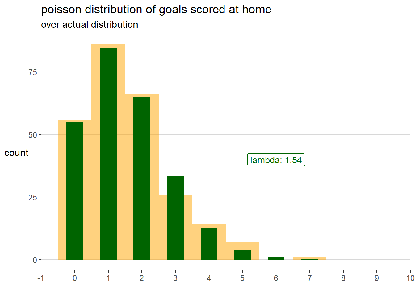
The goodness of fit for the home goals distribution is confirmed by a very high p value equal to 0.4684794.
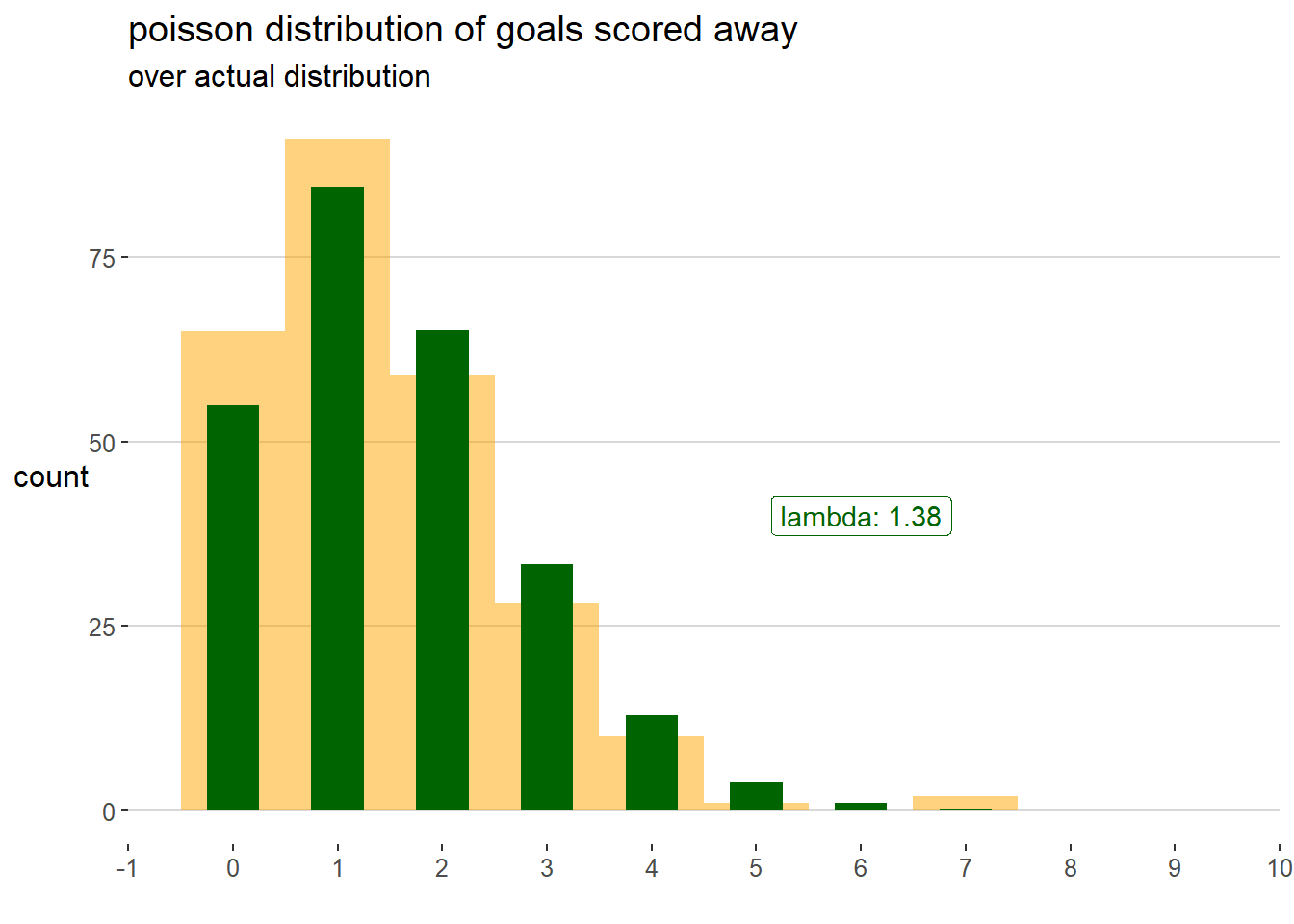
The goodness of fit for the away goals distribution is confirmed by a very high p value equal to 0.9887426.
parameters for Monte Carlo simulation
Reasonably assuming Poisson distribution is a good fit for the goals scored and conceded, a table with all parameters needed for the Monte Carlo simulation is build. This table include the following parameters:
average goals scored at home (avgHGS);
average goals conceded at home (avgHGC);
average goals scored away (avgAGS);
average goals conceded away (avgAGS);
defense home modifier (defHmod) computed as the ratio between the average goals conceded at home by the club over the overall average goals conceded at home;
defense away modifier (defAmod) computed as the ratio between the average goals conceded away by the club over the overall average goals concede away.
Table 3: parameters for monte carlo simulation
club
avgHGS
avgHGC
avgAGS
avgAGC
defHmod
defAmod
Atalanta
2.750
1.583
2.846
1.154
1.152
0.750
Bologna
1.385
1.538
1.538
1.692
1.119
1.100
Brescia
1.000
1.923
0.692
1.846
1.399
1.200
Cagliari
1.923
1.769
1.333
1.417
1.287
0.920
Fiorentina
1.000
1.308
1.462
1.462
0.951
0.950
Genoa
1.167
1.500
1.214
2.071
1.091
1.346
Inter
1.917
0.833
2.000
1.077
0.606
0.700
Juventus
2.385
0.769
1.462
1.077
0.559
0.700
Lazio
2.786
0.714
1.750
1.083
0.519
0.704
Lecce
1.462
2.000
1.154
2.308
1.455
1.499
Milan
1.000
1.154
1.154
1.462
0.839
0.950
Napoli
1.308
1.385
1.846
1.385
1.007
0.900
Parma
1.308
0.923
1.250
1.583
0.671
1.029
Roma
2.000
1.462
1.923
1.231
1.063
0.800
Sampdoria
1.143
1.571
1.091
2.000
1.143
1.299
Sassuolo
2.154
1.692
1.083
1.417
1.231
0.920
Spal
0.917
1.667
0.643
1.714
1.212
1.114
Torino
0.917
1.833
1.308
1.769
1.333
1.150
Udinese
0.769
0.923
0.846
1.923
0.671
1.250
Verona
1.417
1.000
0.923
1.077
0.727
0.700
simulated final results
Running the simulation 100 times drawing goals from the Poisson distribution where \(\lambda\) is the average goals scored by the home or away team scaled by the defense away and defense home modifier respectively
the following final standings has been predicted.
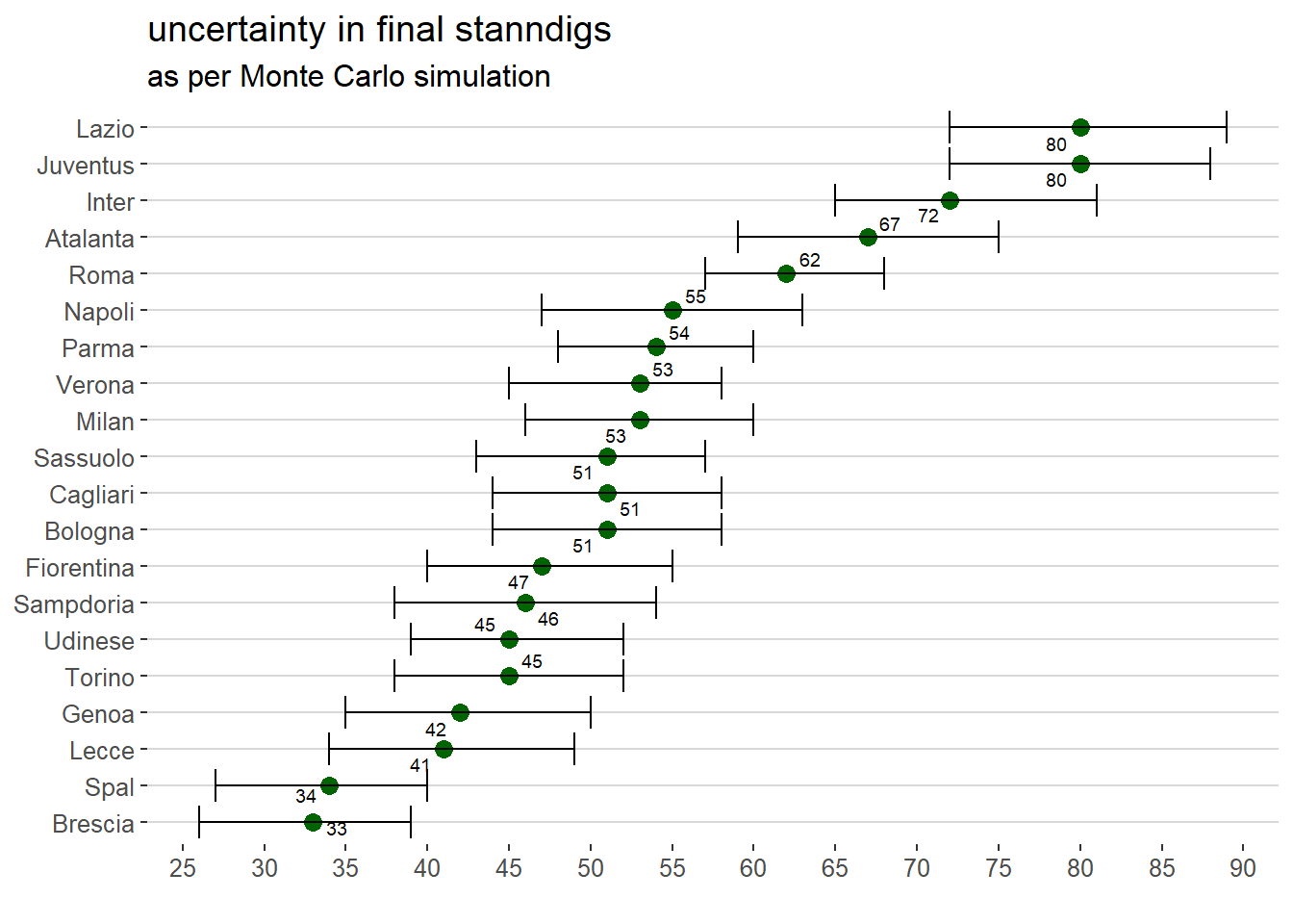
The final standings above highlights the uncertainty in the final outcome propagated from the Poisson distributions of goal. This Monte Carlo simulation shows the average points and also their confidence interval at 90% confidence level.
It shows also that Lazio could have been the winner and that not all positions are predetermined by the demonstrated abilities in the first part of the season.
which Team would have been the winner?
As per the 3 models above, the “scudetto” (or championship) was a matter of 2 clubs only: Juventus and Lazio. Juventus had a slight advantage in points achieved even if not reflected in the win expectations and in the club abilities according to Davidson model so Lazio chances of contending for victory was good.
Now that the championship restarts after a long period of stop no one can say anything about the current status of club abilities so it is really difficult to predict final results. The Author suggests to come back and read this post again when actual championship end just to check if any significant changes will occur.
As a side note please consider the effort of the Author, an irrational football fan, to stick to data science only while writing this post.
Feel free to email me if you would like to delve into analysis details, thanks for reading!
The analysis and simulations shown in this post have been executed using R as main computation tool together with its gorgeous ecosystem. In particular Davidson modeling relied on “gnm” and “BradleyTerry2” packages. “doParallel” package allowed to quickly perform the Monte Carlo simulation.
Davidson, Roger R. “On Extending the Bradley-Terry Model to Accommodate Ties in Paired Comparison Experiments.” Journal of the American Statistical Association, vol. 65, no. 329, 1970, pp. 317–328. JSTOR, www.jstor.org/stable/2283595.↩︎