
the risk of getting involved in a road accident has been forgotten during COVID pandemic. The goal of this post is to remember that this risk is still present and will become more and more evident as people resume moving on the road.
analysis intro
In 2020, Istat (Italian Institute for Statistics) reported the record collapse of accidents, injuries and victims on Italian roads. According to a preliminary estimate, from January to September - thanks to the restrictions due to the Covid pandemic - accidents with injuries to people were 90,821, equal to -29.5% compared to the previous year. The injured were 123,061, with a decrease of 32%, while the victims within the thirtieth day were 1,788, with a decrease of 26.3%. If the observation is limited to the period January-June 2020, the decreases are more pronounced, amounting to about 34% for victims and almost 40% for accidents and injuries. ansa.it
Since people wants to go back to before the pandemic began, the analysis takes into account data on road accidents in Italy in 2019, the last year without COVID so far. Exploring this data, a terrific amount of accidents and related injuries and deaths are reported.
2019 road accidents
The Automobile Club of Italy aka ACI, a Federation of 103 Automobile Clubs which represents and protects the interests of Italian motoring, of which it promotes the development through the dissemination of a new culture of mobility, publishes incidentality data for 2019 on its open data website
The total numbers for accidents, consequent deaths and injuries are impressive. in 2019 before the pandemic restricted traffic on the streets, there was accidents, deaths and injuries as per table.
| year | accidents | deaths | injuries |
|---|---|---|---|
| 2019 | 172,183 | 3,173 | 241,384 |
On an average day of 2019 it was possible to count about 474 road accidents, 8 deaths and 661 injured people.
incidentality geo distribution
With the help of a choropleth map, it is possible to identify where in Italy the road accidents occur the most.
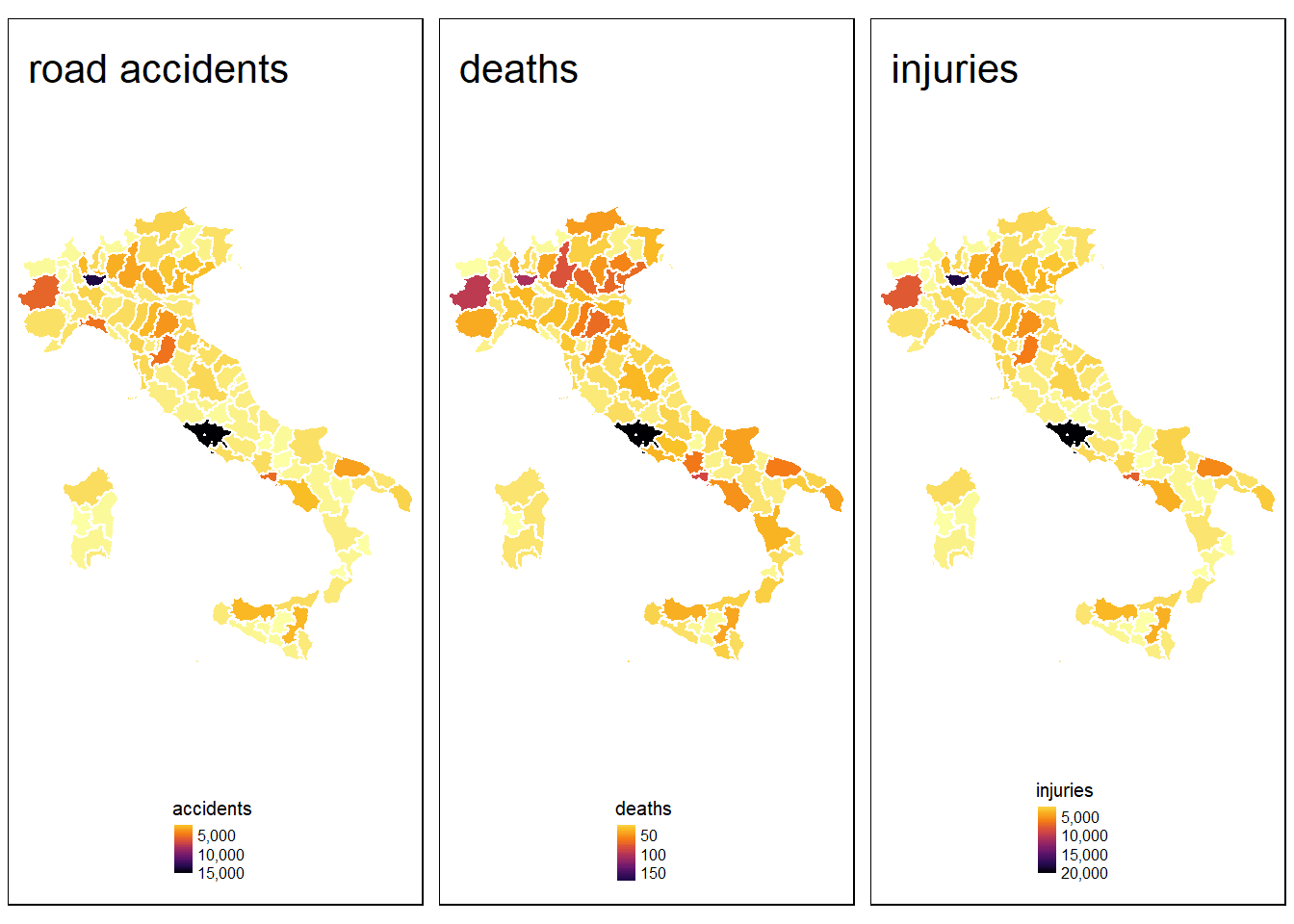
At first glance it seems that the occurrence of road accidents varies greatly depending on the geographical location in Italy.
The map shows by means of color intensity the quantity of the phenomenon in a territorial unit called Supra-municipal Territorial Unit (UTS), an administrative unit that groups together several municipalities and is part of a region. In this post from now on UTS is referred to as district. The district boundaries shapefiles are provided by Istat
the best districts …
The following infographic shows the best district by road accidents, related deaths and injuries, i.e. the districts with less events.
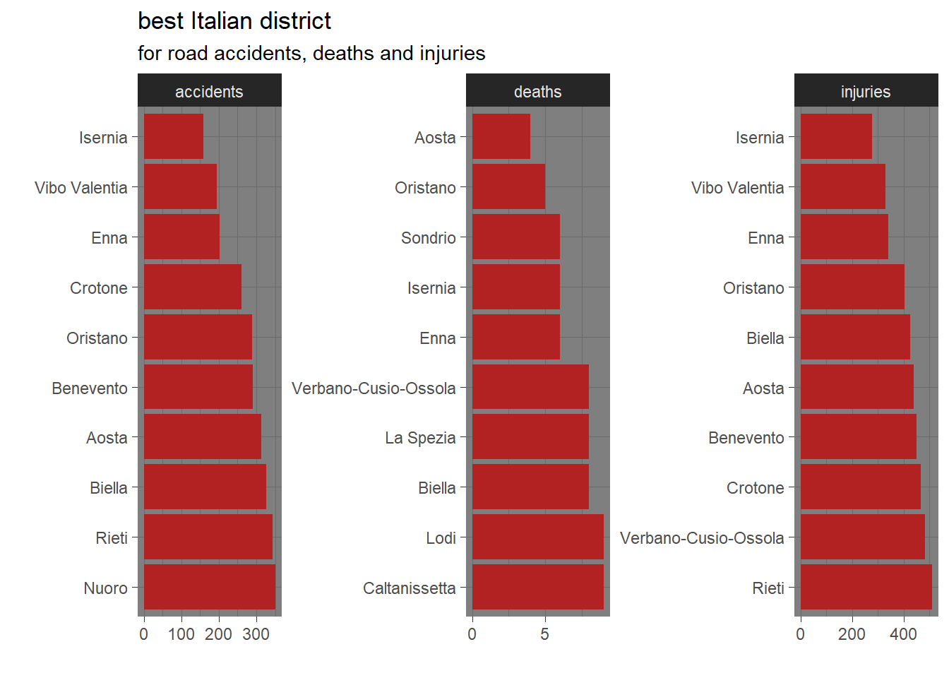
The district counting less road accidents is Isernia in the south of Italy that is also the less populated ditrict in Italy. Also Vibo Valentia, Crotone, Benevento are located in the south. Oristano, Nuoro, Enna are districts in the big islands territory of Sardinia and Sicily. Aosta and Biella are in the north of Italy while Rieti is in the center of Italy. Aosta had the least number of deaths related to road accidents perhaps due to the mountainous conformation of its territory.
… and the worst ditricts
coming to the bad side, the visualization below shows the 10 worst districts by road accidents, deaths and injuries.
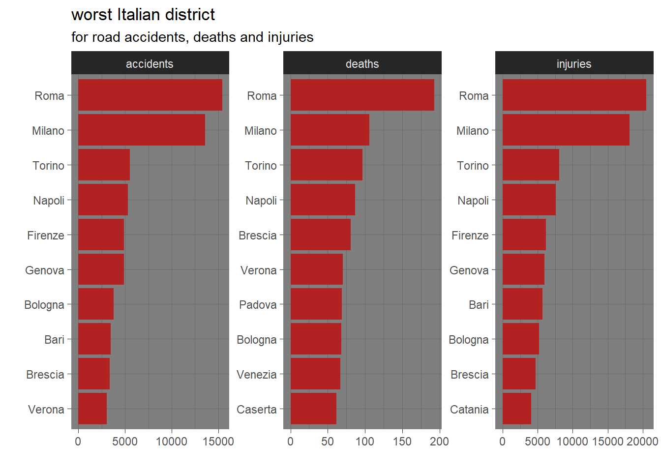
The worst ranks are deserved by the big metropolitan areas such as Rome, Milan, Turin and Naples. It is worth noting the presence of districts that are also regional capitals: Genova, Firenze, Bologna, Bari.
modeling road accidents
In order to explain what drives the occurrence of road accidents two modeling approaches:
model road accidents taking in consideration explanatory variables without accounting for geographical distribution
model accidents geographically
The first approach is to adapt a global linear model that captures the association of accidents with structural differences between districts. The higher frequency of road accidents is reasonably associated with the resident population, registered vehicles, the number of municipalities within a district and the area of the district.
The geo approach can help in understanding why road accidents occurs where they do or at least in examining the way in which the relationships between road accidents and the set of explanatory variables might vary over space.
The steps include:
explore road accident overall distribution
explore explanatory variables
evaluate the global model
evaluate the geographic model
accidents overall distribution
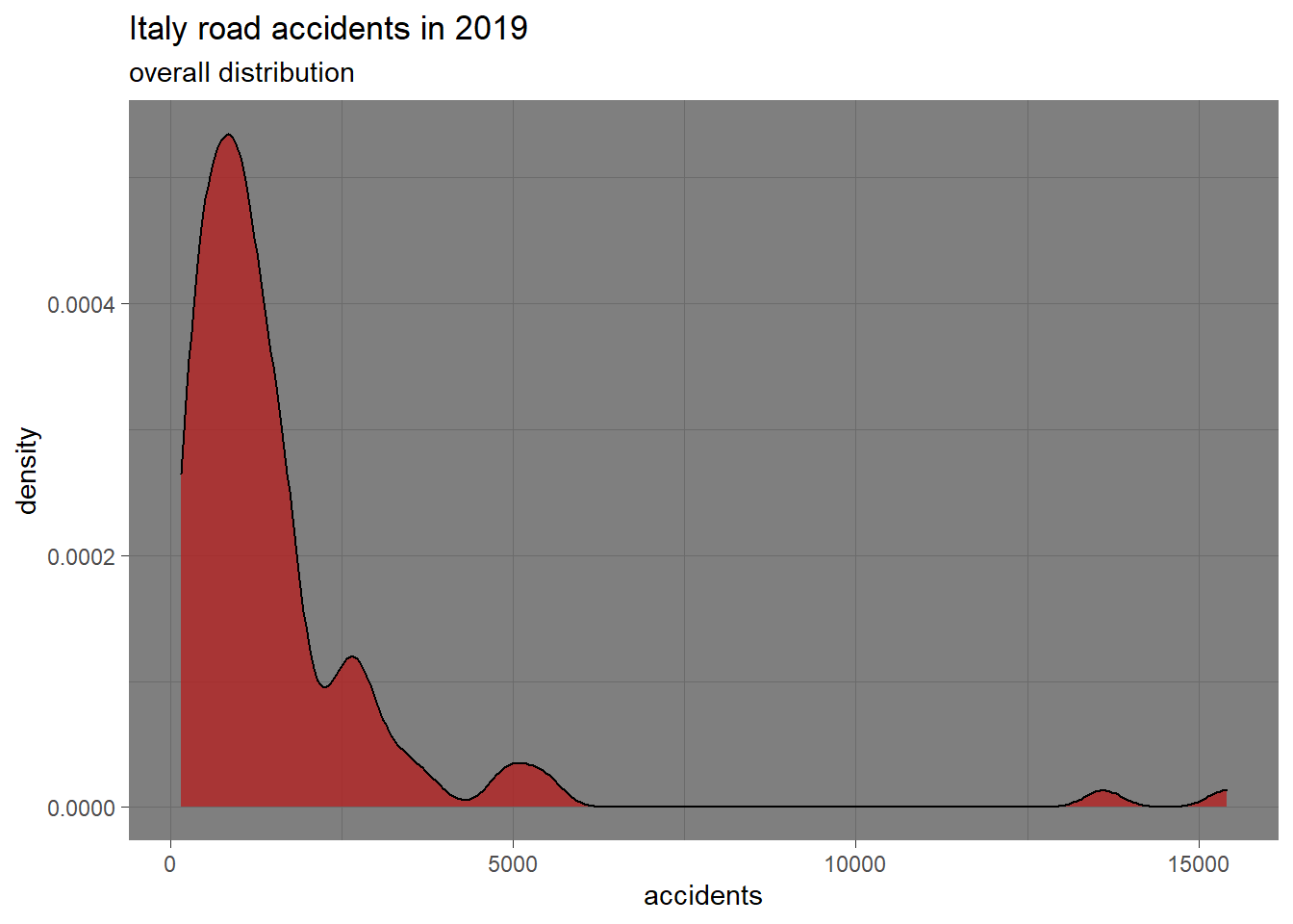
The distribution shows to be right skewed with big outliers in correspondence with Rome and Milan districts.
explanatory data
For this post modeling attempt 4 explanatory variables are considered:
resident population that measures how much the district is populated
district area that measures how wide is the district
number of municipalities in a district that may reflect the complexity of the road network within a district
district vehicles fleet, the quantity of vehicles registered in the district independently from their category (cars, motorbikes, bus, truck, …).
The data have been retrieved from scraping the page Province Italiane per Abitanti but the last one that has been downloaded from the open data site of ACI.
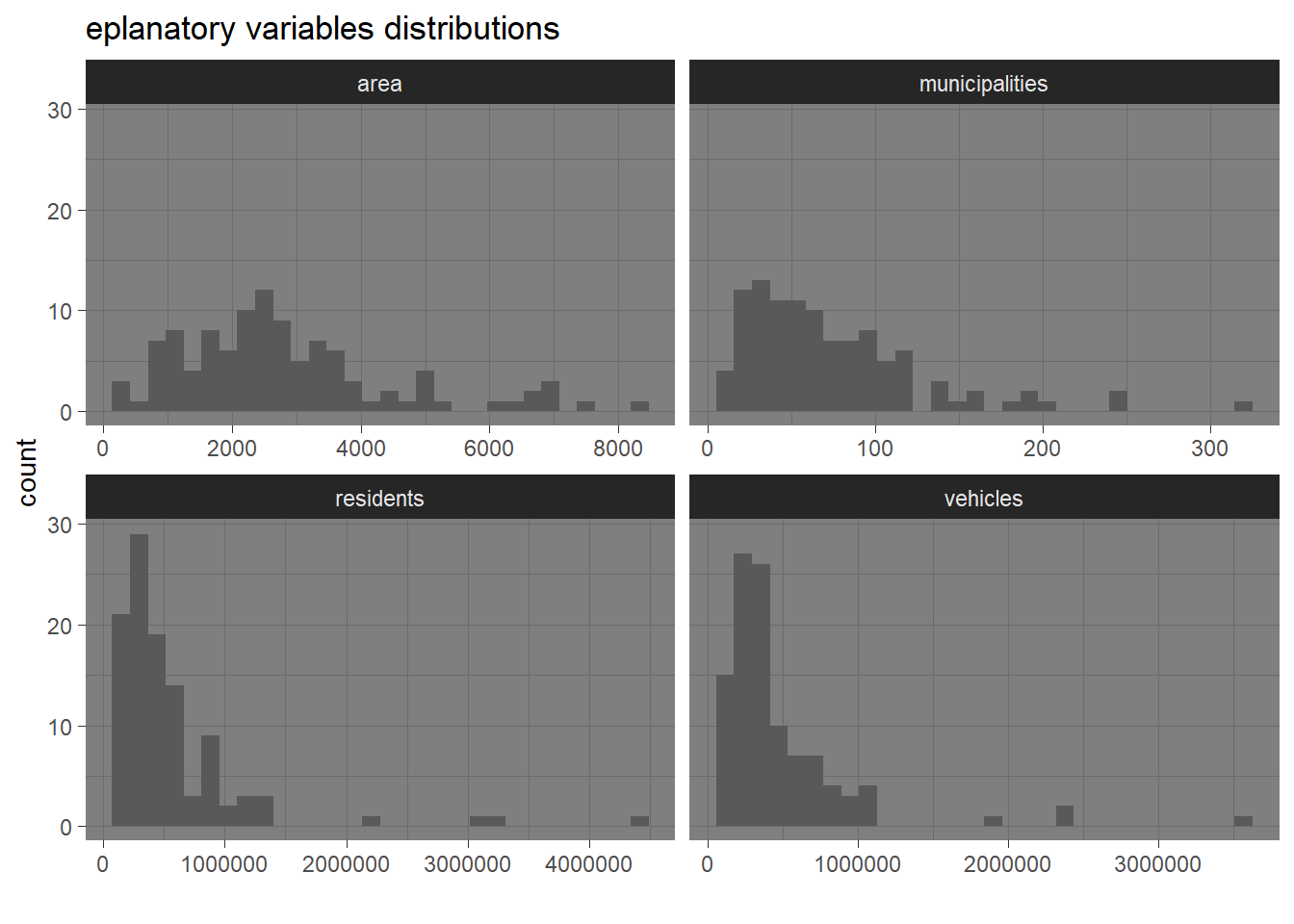 It is worth noting the similarity in the distribution between area and municipalities and between residents and vehicles.
In particular considering the ratio of vehicles per resident it is possible to count 8 districts with more vehicles (including all motorized category) than people.
It is worth noting the similarity in the distribution between area and municipalities and between residents and vehicles.
In particular considering the ratio of vehicles per resident it is possible to count 8 districts with more vehicles (including all motorized category) than people.
| district | region | vehicles_resident_ratio |
|---|---|---|
| Aosta | Valle d’Aosta | 2.31 |
| Trento | Trentino-Alto Adige | 1.61 |
| Sassari | Sardegna | 1.29 |
| Bolzano | Trentino-Alto Adige | 1.21 |
| Nuoro | Sardegna | 1.20 |
| Firenze | Toscana | 1.06 |
| Isernia | Molise | 1.05 |
| Catania | Sicilia | 1.01 |
Furthermore the average vehicles to resident ratio equals 0.9.
Residents and Vehicles variables are highly correlated with the quantity of road accidents as shown by the scatter plots below
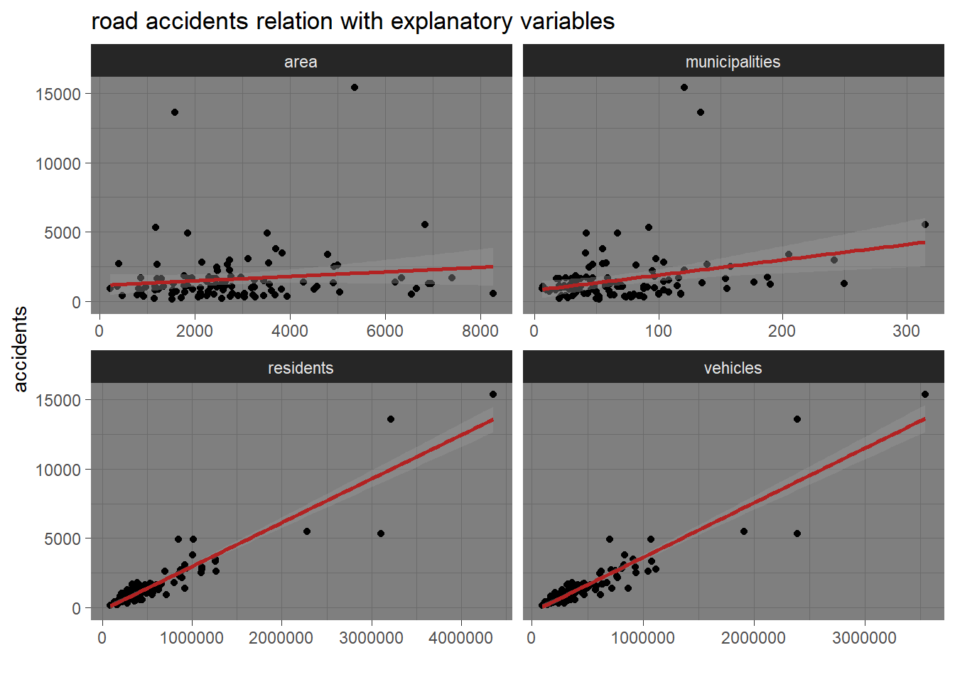
and the following correlation plot.
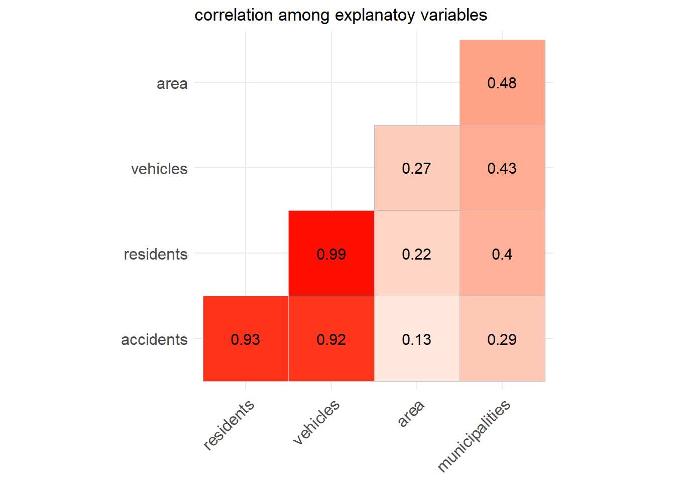
Explanatory variables residents and vehicles are almost colinear so only residents is used a indipendent variable.
global linear model
As stated above, the first modeling attempt consists in fitting a linear model in which the road accidents are regressed against the explanatory variables as per the following formula. \[accidents \sim b_{intercept} + b_{res}\cdot residents + b_{mun}\cdot municipalities + b_{area}\cdot area + \epsilon\]
where the fitted coefficients are reported in the following table:| term | estimate | std.error | statistic | p.value | conf.low | conf.high |
|---|---|---|---|---|---|---|
| residents | 0.0033047 | 0.0001296 | 25.504723 | 0.0000000 | 0.0030477 | 0.0035617 |
| municipalities | -3.0122996 | 1.6327314 | -1.844945 | 0.0679188 | -6.2504373 | 0.2258381 |
| area | -0.0637890 | 0.0496842 | -1.283890 | 0.2020610 | -0.1623259 | 0.0347478 |
Residents coefficient is statistically significant at 99% confidence level while municipalities is statistically significant at 90%. The coefficient for residents says that 1000 more residents in a dis6trict leads to about 3 more road accidents holding all other variables constant.
Some problems about this model have been already highlighted such as the right skewed distribution of the dependent variable due to actual data for metropolitan areas or the high correlation between residents and vehicles variables managed by using only residents as explanatory variable.
In order to check for further problems diagnostic plots are visualized below.
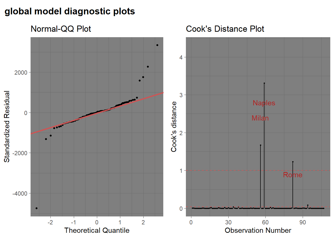 Checking above diagnostic plots two more main assumptions for linear model validity are not completely satisfied:
normal qqplot shows a significant deviance of residuals from normality in the queues;
the Cooks Distance plot indicates the presence of at least 3 districts (Naples, Milan and Rome) that can have too much influence in determining the model parameters.
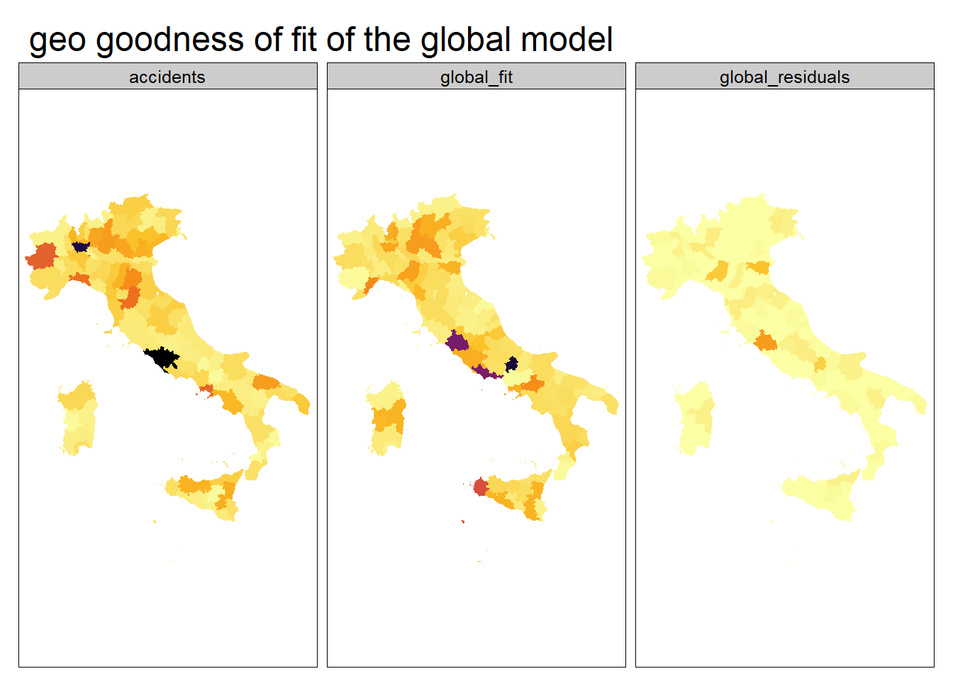
Nonetheless the adjusted R square measure of goodness of fit indicates that 0.871 of road accidents variability is explained by the model and computing the RMSE (Root Mean Squared Error) from the model residuals the error is on average equal to \(\pm\)740 accidents.
The goodness of fit related to the geography can be analyzed visualizing the actual geo distribution of the accidents against the fitted value by the global model together with the geo distribution of the residuals.
spatial regression
Even if there’s no specific indication that there is a neighborhood effect among districts related to the considered variables (test for spatial autocorrelation does not reject the null hypothesis), the second modeling attempt consists in fitting a spatial lag model. The spatial lag regression model is a model that considers explanatory variables on an area with other areas associated with it (and not considering error spatial dependency). In order to interpret the regression coefficients correctly in a spatial lag model, direct and indirect effects of each variable has to be considered.| variable | direct | indirect | total |
|---|---|---|---|
| residents | 0.0032787 | -0.0004527 | 0.0028261 |
| municipalities | -4.1238882 | 2.8631853 | -1.2607029 |
| area | -0.0338238 | -0.1365895 | -0.1704133 |
The direct effect refers to the local effect while the indirect one accounts for spill-over, and the total effect of a unit change in each of the explanatory variables.
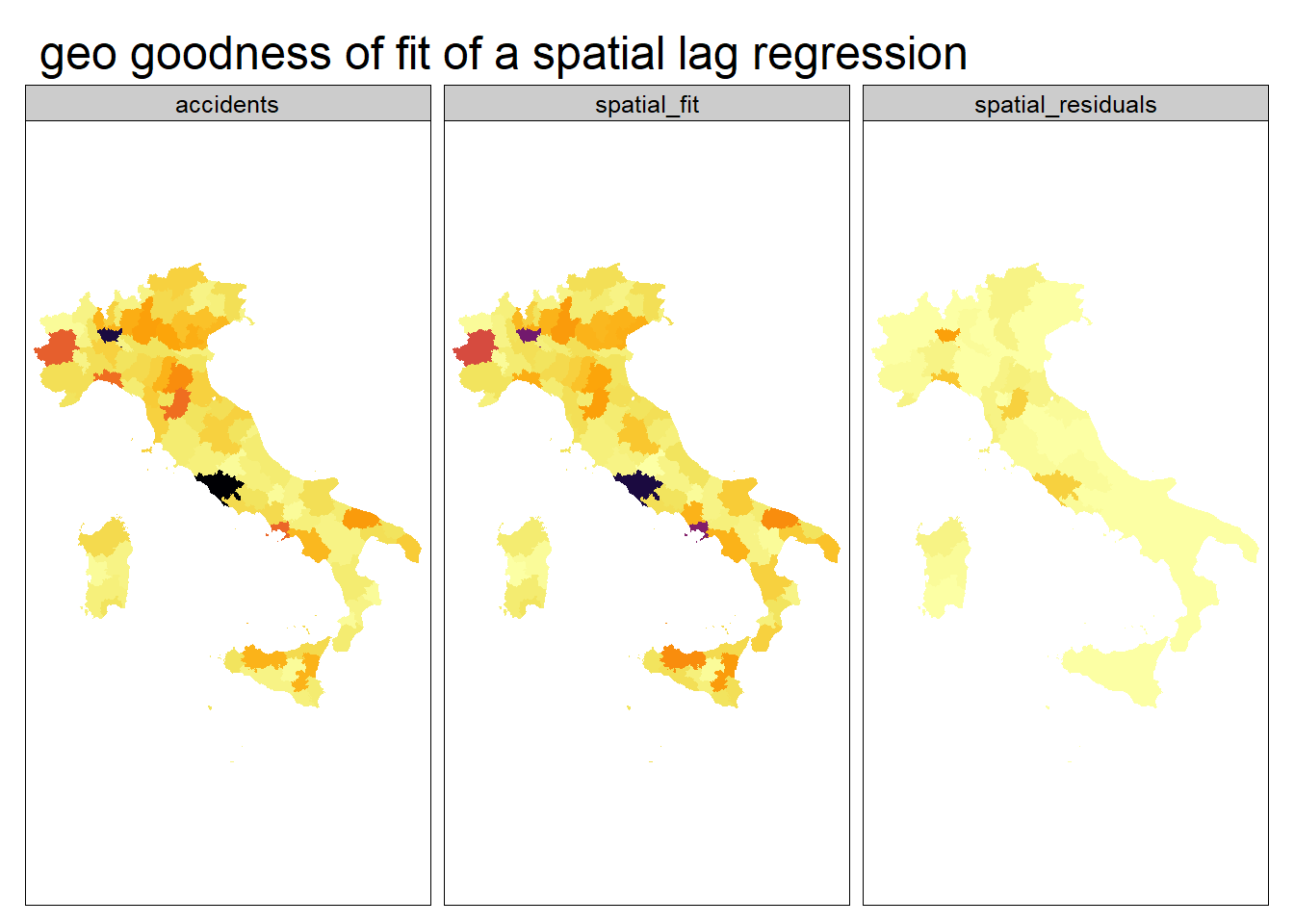
Using the spatial lag regression the overall goodness of fit remains almost unchanged: the spatial adjusted r squared is 0.874 not so different from the global one, 0.871. Furthermore the RMSE improves by more than 20 units being equal to 720.
The real gain of the spatial model is that fits better the geographic distribution as shown in the below plot.
conclusion
The exploratory data analysis and the modeling attempt lead to the following final considerations:
the road accidents and related injuries and deaths were an heavy issue in Italy during 2019 especially in district such as Rome and Milan;
district vehicles fleet dimension is terrific;
a global model (i.e. a model that don’t take in consideration the geography) explain more than 80% of the variability in road accidents but does not fit very well for district such as Rome, Milan and Naples;
given that a better local fit is achieved using spatial regression, it is possible to say that there’s something specific in the geographic localization that explain why road accidents occurs where they do.
As a general final consideration it can be stated that not all of the effects of COVID pandemic have been negative: the decrease in road accidents is a clear example.
The author doesn’t understand why people so badly want to go back to the previous situation (pre COVID) and he thinks that the pandemic should represent an opportunity to rethink people’s way of life!
Feel free to email me if you would like to go deeper in the analysis, thanks for reading!
The analysis shown in this post have been executed using R as main computation tool together with its gorgeous ecosystem ( tidyverse included). In particular geographic analysis was based on sf , spdep and spatialreg packages.