
Everyone is able to make money trading by applying a buy and hold strategy when market is bullish, but when times get tough …
choices
Investors have the following choices:
exit from trade avoiding more potential losses
hold their positions believing their portfolio is so robust to overcome the crisis
try alternative trading strategies
This post try to assess simple signal based strategies through a simple yet not so realistic backtesting.
backtesting setup
Backtesting is a trading simulation accomplished by reconstructing, with historical data, trades that would have occurred in the past using rules defined by a given strategy.
In order to keep simulation simple as in a blog post it can be, it is assumed that:
only NASDAQ Composite index ETF can be traded
investor can alternatively invest on or completely disinvest
only one daily trade is allowed
decisions on next day trade are taken on the basis of ETF data of that day and previous days
trade daily return can either be the index daily return when capital is invested or 0 if capital is disinvested
only long (buy low sell high) position are allowed
trading strategy cannot be changed over simulation time
investor does not incurr in any transaction costs
capital gain taxation is not cosidered
backtesting data
data collection
Data for this trading simulation include only:
- NASDAQ Composite index (symbol “^IXIC”)
| date | open | high | low | close | volume | adjusted |
|---|---|---|---|---|---|---|
| 2000-01-03 | 4186.19 | 4192.19 | 3989.71 | 4131.15 | 1510070000 | 4131.15 |
| 2000-01-04 | 4020.00 | 4073.25 | 3898.23 | 3901.69 | 1511840000 | 3901.69 |
| 2020-04-22 | 8434.55 | 8537.31 | 8404.54 | 8495.38 | 3025060000 | 8495.38 |
| 2020-04-23 | 8528.84 | 8635.23 | 8475.20 | 8494.75 | 3734720000 | 8494.75 |
| 2020-04-24 | 8530.08 | 8642.93 | 8464.42 | 8634.52 | 3673170000 | 8634.52 |
Data are collected from year 2000 in order to have enough data to train simple machine learning model but the backtesting is focused on years 2019 and 2020.
The data source is Yahoo Finance.
exploring data
The bars chart of NASDAQ Composite prices highlights that after February 24 when COVID-19 outbreaks in Italy:
the price trend decreased till a max drawdown on middle March and then increased
volumes were always sustained
price bars have been generally wider that before (larger open close price difference)
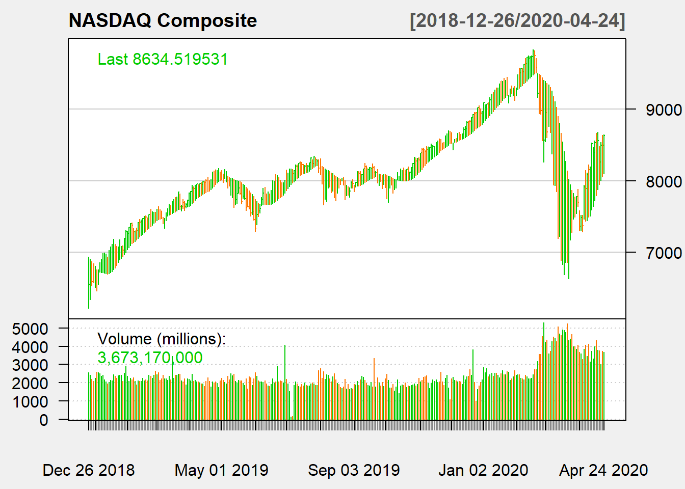
Market volatility is not necessarily negative seen by a trader having the ability to predict the direction of the price move. Investors can significantly profit of this situation entering in certain highly rated positions when prices are very low and professional traders can profit also shortening some positions.
NASDAQ returns
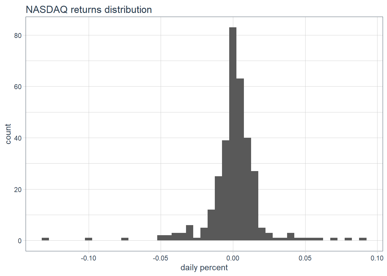
The histogram of realized returns from 2019 till post publication date shows that the distribution is:
centered around 0;
left skewed (more mass in the negative side);
presenting long tail in particular in the negative direction.
| ArithmeticMean | 0.0008 |
| GeometricMean | 0.0006 |
| Kurtosis | 13.0080 |
| LCLMean(0.95) | -0.0012 |
| Maximum | 0.0893 |
| Median | 0.0015 |
| Minimum | -0.1315 |
| NAs | 0.0000 |
| Observations | 334.0000 |
| Quartile1 | -0.0041 |
| Quartile3 | 0.0077 |
| SEMean | 0.0010 |
| Skewness | -1.1026 |
| Stdev | 0.0187 |
| UCLMean(0.95) | 0.0028 |
| Variance | 0.0003 |
In particular kurtosis is quite high indicating much more returns in tails than in normal distribution.
Visualizing returns versus time it is possible to identify the time slot in which volatility grows drammatically in corrispondence with COVID-19 pandemic outbreak.
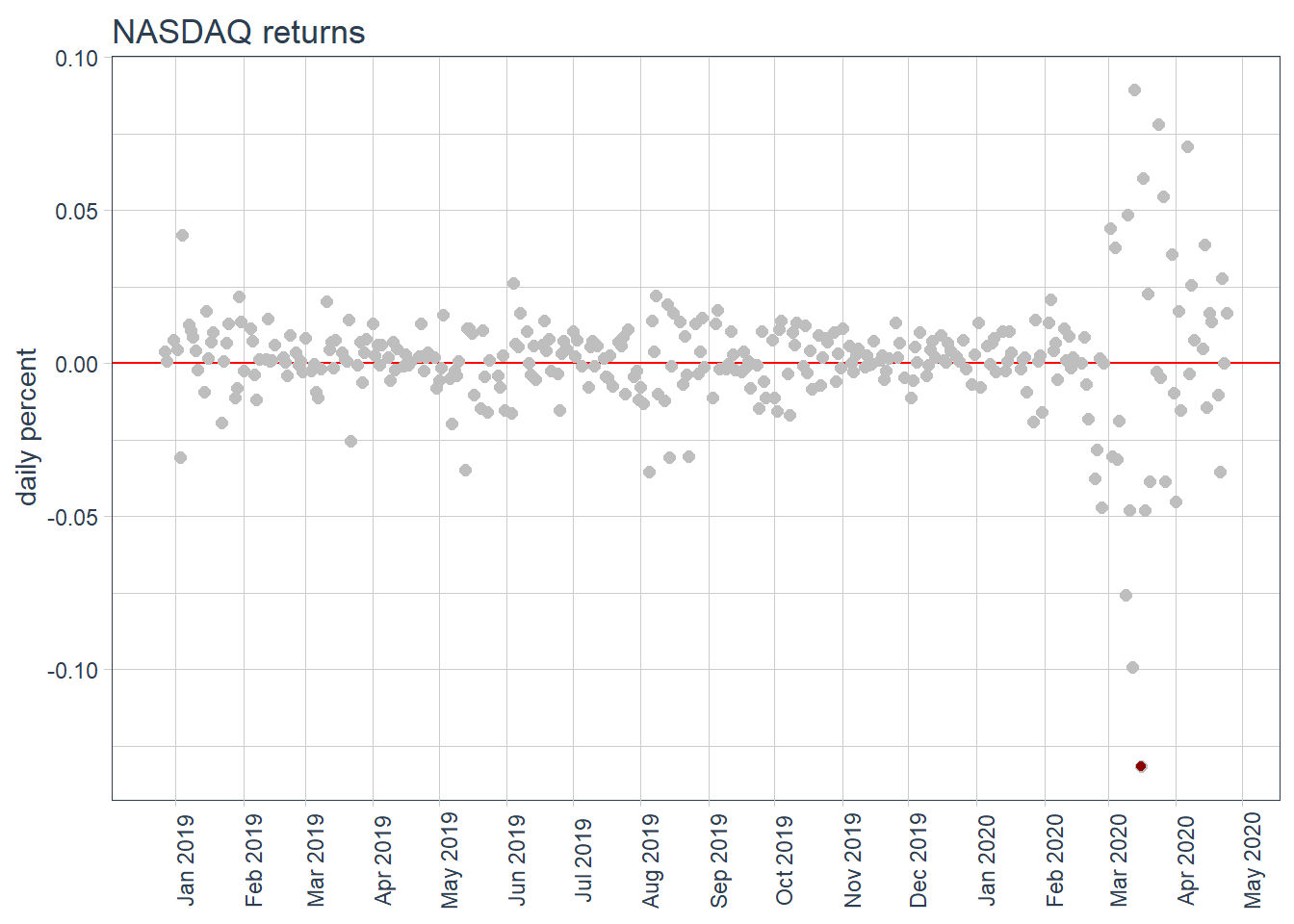 Plotting NASDAQ Composite returns point out the max drawdown occurred on March 15 when returns went down 0.13 % in one day.
In order to check for any clue of the crisis, rolling standard deviation on a short window of 10 days is plotted against time.
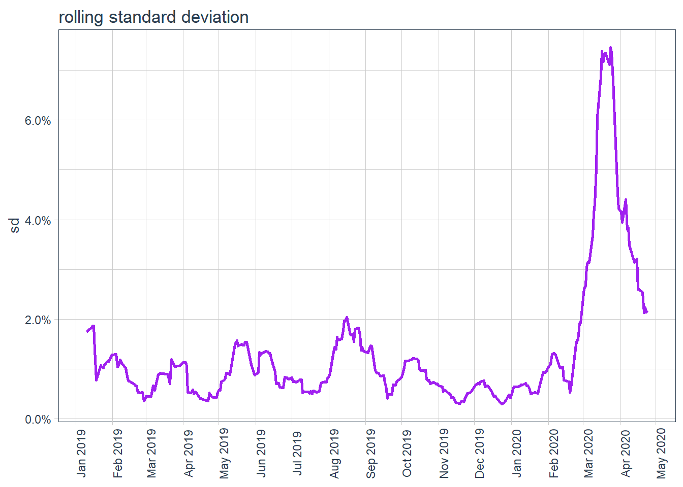
No clear clues of standard deviation rise is present before February 24.
trading strategies
After acklowledging that nothing in market data could have warned about change in volatility regime, it is of interest understand which kind of trading strategy would have profit the most also with this dramatic change in market behavior. Three strategies are compared with buy and hold one where buy occurred in January 2019.
The first strategy, let’s call it “down up”, is based on the idea that after 3 consecutive daily market move downwards within 5 days, a rolling week window, price is likely to go up and investors could profit selling after 2 days move upwards in next 5 days. It is a so called heuristic with no sounding math theory behind. Furthermore it has been optimized over all the simulation data so no clue about how this strategy performs on unseen data.
The second strategy, let’s call it “moving averages”, is based on detecting signals for fast and slow moving averages crossing so that investor buy when fast moving average is above the slow moving average, while he sell when fast moving average moves below the slow one. For this simulation fast moving average considers a time window of 5 days while the slow one considers 20 days.
The third strategy, let’s call it “predicted next move”, is based on the possibility to predict next day market move using simple machine learning algorithm that simulates having a not so good trading advisor.
simulate down-up strategy
Implementing down-up strategy specified as buy only after 3 consecutive downs and sell after 2 ups, the difference in growth in respect to buy and hold is remarkably positive provided the simulation assumpion of no transaction costs.| date | buy and hold | down up | delta |
|---|---|---|---|
| 2020-04-23 | 1.216 | 1.358 | 0.142 |
Charting this strategy results starting from early January 2019, it is clear that down-up strategy has always performed worse till actual tough time begins.
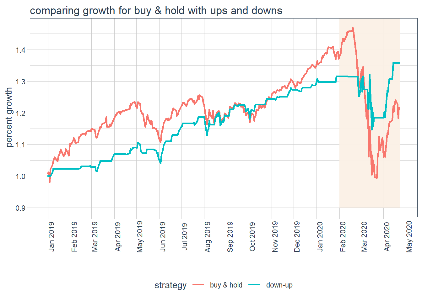 This strategy infact smoothed market wins but also avoided deep losses therefore it protects better investor capital.
implementing moving averages strategy
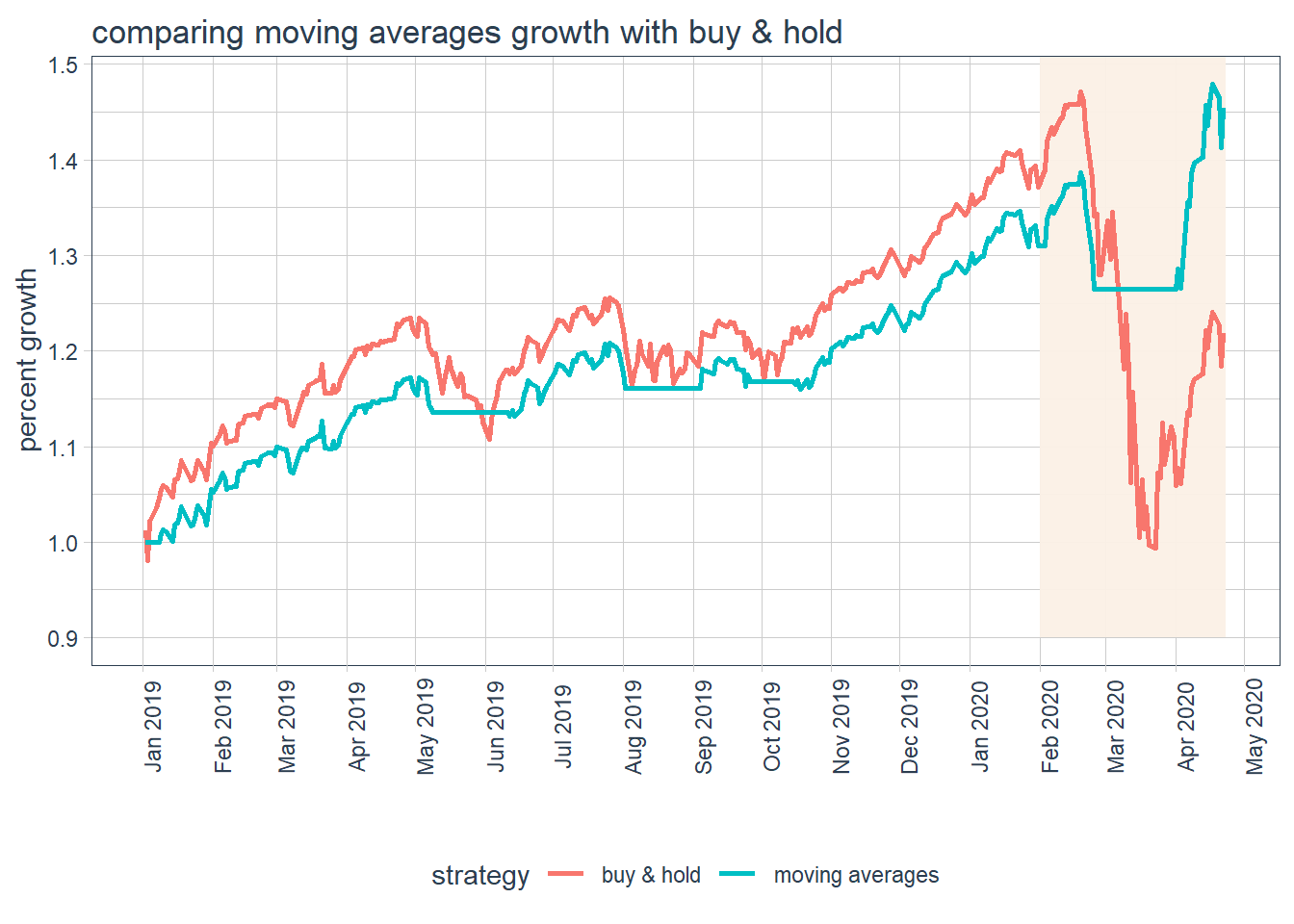
The moving averages strategy performed even better to date.| date | buy and hold | moving averages | delta |
|---|---|---|---|
| 2020-04-23 | 1.216 | 1.451 | 0.235 |
Chart of moving averages strategy results compared with buy and hold ones shows that the moving averages strategy mimics buy and hold when market is bullish but allows to exit from trade whenever the price trend is continuously decreasing and to re-enter whenever trend change.
strategy predicting up & down of next day
When J.P. Morgan was asked what the market will do he responded in three simple words. “It will fluctuate.” He has been proven correct time and time again. But he avoided the investment relevant question: will it fluctuate up or down?
kNN predictive model
In order to predict the movement of the market, the kNN, k Nearest Neighbours, algorithm has been selected from the vast toolset of predictive modeling.
k Nearest Neighbors is a non-parametric classification method that make use of distance (or similarity) measures. In particular for numerical predictors the euclidean distance is used. Euclidean distance is the length of the segment connecting 2 data points in the predictor space and it is defined as:
\[d(\overrightarrow{x}^{(i)},\overrightarrow{x}^{(j)}) = \sqrt{(x_1^{(i)}-x_1^{(j)})^2+(x_2^{(i)}-x_2^{(j)})^2+...+(x_p^{(i)}-x_p^{(j)})^2}\]
The kNN algorithm stores all the data and classify new data points in relation of majority of k nearest (as per euclidean distance) points class.
feature engineering
The attempt to predict the next market move for NASDAQ index is performed using the following engineered predictors:
volume discretized quartile for the day and for previous 5 day
scaled closing price for the day and the previous day
slow and fast moving averages of price
scaled open price for the day
price candle up/down for the day and previous 5 days
day of the week (Mon, Tue, …)
In order to train the model the response class is engineered as the up or down movement for the next day.
model training and evaluation
The kNN model has been trained on data preceding January 2019 and tested on data from that date onward.
The following table represent the confusion matrix related to the simulation data (from January 2019 till post publication date)| 0 | 1 | |
|---|---|---|
| 0 | 88 | 97 |
| 1 | 59 | 86 |
The overall test accuracy is 0.53, only slightly better than a random guess and not reaching the performance of the base model 0.55, i.e. predicting always the majority class.
Using more training data and trying different non linear classification model could increase overall test accuracy. But the objective of this model is to simulate trading decisions that a trader can take based on his historical experience of the market so no effort will be spent for increasing model predictive performance.
applying predict next move strategy
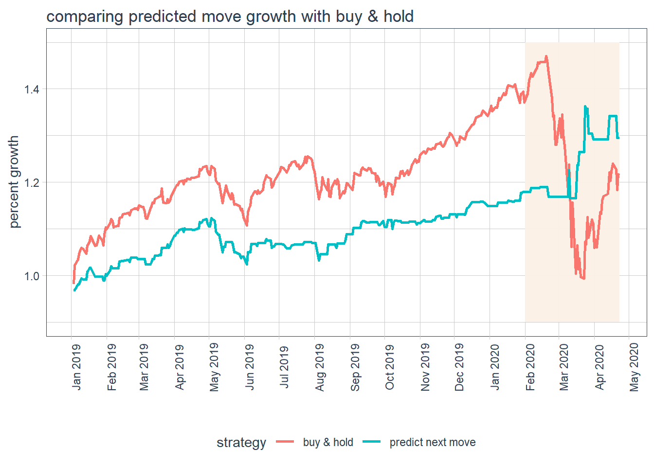
Nontheless applying a strategy based on predicted value, buy when predicted move for next day is up and sell when the move is predicted in the opposite direction, seems to outperform buy and hold strategy during high volatility period while it clearly underperforms in stable market conditions.
| date | buy and hold | next move | delta |
|---|---|---|---|
| 2020-04-23 | 1.216 | 1.295 | 0.079 |
Visualizing this strategy along all the simulation timeframe it is evident that it did not performed well during bullish market period but when volatility went high this strategy can profit of daily price move.
Having a well validated model with good accuracy would make this strategy really interesting in high volatility period.
trading in troubled times
Plotting the 4 strategies together for year 2020 points out that:
all alternative strategies outperformed buy an hold from middle March
down-up strategy incurred in losses during price went downward fast but much slower than buy and hold
moving averages strategy was less sensible to quick market move so it truncated losses and start profit from favorable trand just few days after consistent change in market direction
predicted move strategy succeded in make profit from rapid move in prices even if not consistently due to the poor predictive model performance
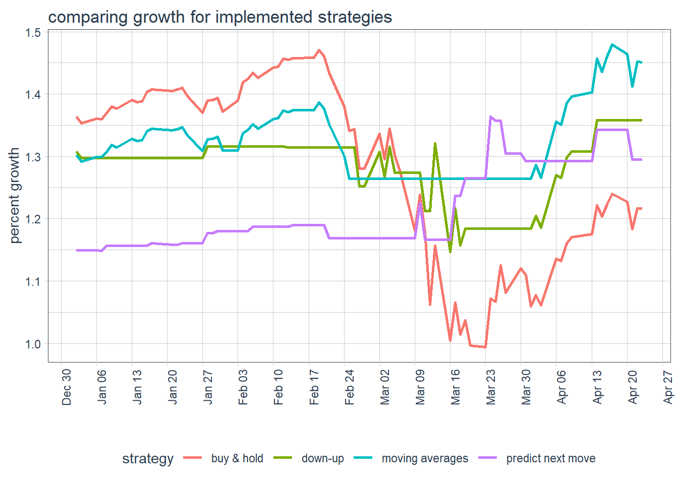
Focusing on particular days it is even easier to visualize the different performances of the trading strategies.
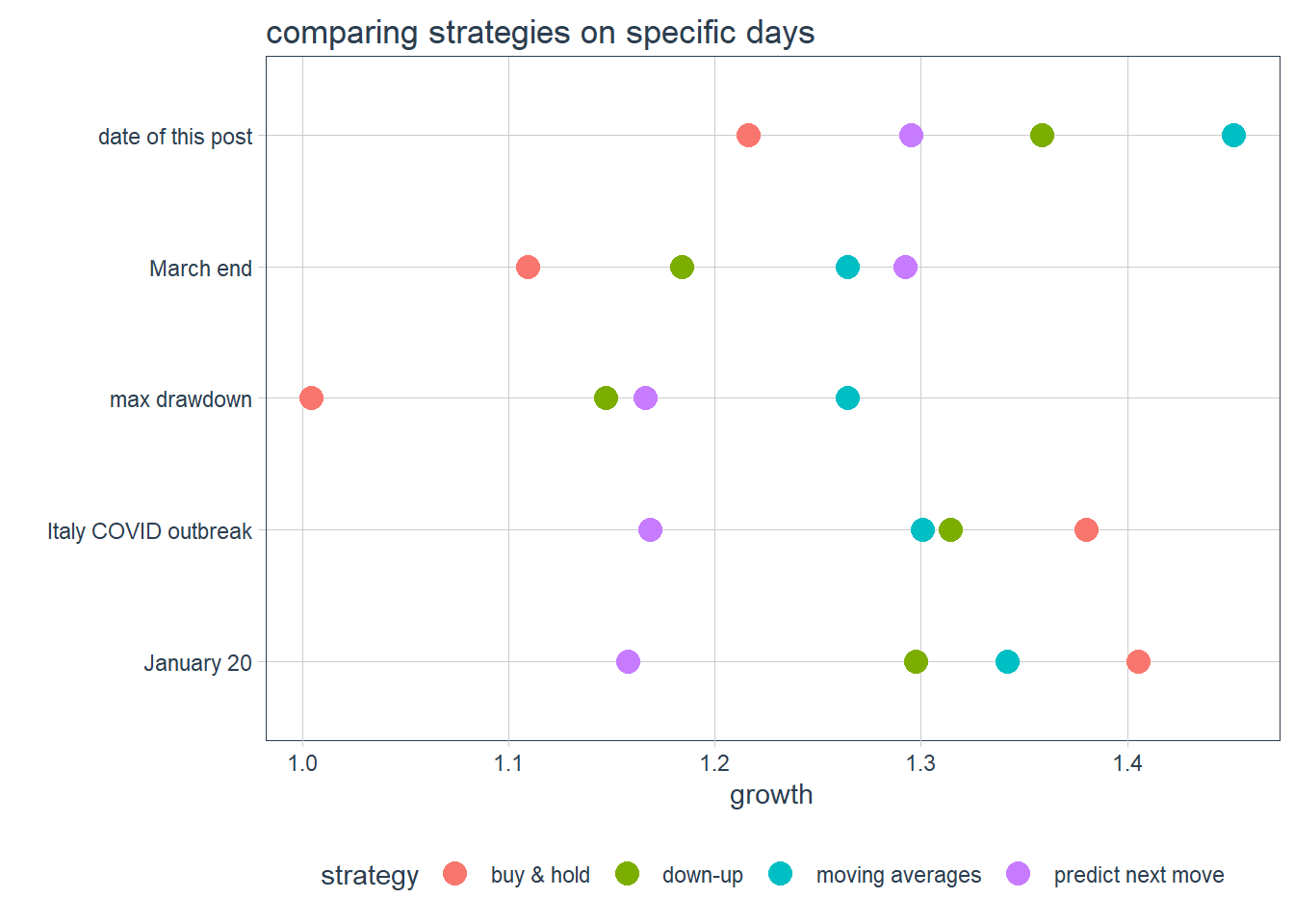
Each specific day shows a different ranking for strategies thus indicating that performances may continuously vary in a high volatility market. So it is really hard to establish a go to strategy among the considered ones.
trading considerations
Following considerations come directly from the quantatitative analysis in this post:
trade is for people with strong nerves;
relying on a buy and hold trading strategy in period of high volatility (an elegant way to say “tough time”) couldn’t be the smartest course of action in the short and medium term. In the long period story may differ a lot;
alternative trading strategy could cope better with uncertainty;
predictive modeling could be a valuable support to investment decisions only provided a better test accuracy is achieved;
financial markets are real complex objects and algorithmic trading can find sub-optimal trading solution responding to some patterns in data but when money is at risk better consider also expert judgments, fundamental analysis and trading instinct.
Feel free to email me if you would like to delve into simulation details, thanks for reading!
The analysis shown in this post have been executed using R as main computation tool together with its gorgeous ecosystem. In particular trading analysis relied on quantmod, PerformanceAnalytics, PortfolioAnalytics, timetk, tibbletime and tidyquant packages.